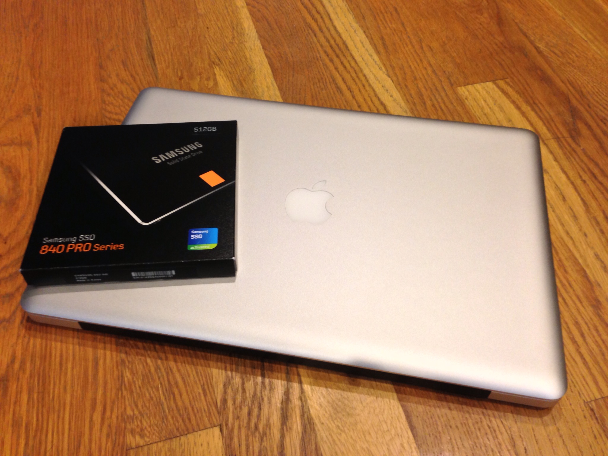
Samsung 840 Pro 512GB SSD Upgrade for my MacBook Pro
This isn’t ostensibly Hyperion related, but I’m going to find a way to tie it back to Hyperion and Essbase. My main machine these days is a MacBook Pro. I love this thing. It’s not even the newest retina model (soon…) but it’s still a beast. Originally it came with a 128GB SSD. I quickly outgrew it – mostly owing to the VMs I store locally. I bumped up to a 256GB Samsung 830 SSD and enjoyed breathing room for awhile longer. Recently, though, I have even outgrown this, owing to various VMs and other files I need on a day to day basis.
I could run my VMs and store files on an external drive, of course. It wouldn’t be too hard to just plug a USB drive. Now, I’m not lazy, but it is just one more thing to deal with (I’m sure performance would be reasonable, but SATA beats USB). This machine has Thunderbolt, but again that’s just one more external thing to plug in and the Thunderbolt enclosures for drives are pretty expensive (i.e., they make more sense for an array of drives rather than just one drive). I could even replace the optical bay (a DVD-RW drive) with a hard drive. This is very tempting – to pop in a 1 TB laptop drive in place of the optical drive. I’m not ready to go there, just yet. After some deliberation, I decided to bump up this baby to a 512 GB Samsung 840 Pro SSD. It’s a little pricey but I’m not ready to commit to a new laptop just yet, gets me the space I need right now, doesn’t entail me having to worry about an external drive, and it is fast. I cloned my existing drive over so this isn’t even new install of the OS or anything. This thing just screams.
How does this relate to Essbase? Well, let me tell you.
Disk performance affects almost all major aspects of Essbase solutions: retrieval times, calc times, data load times, and more. We [database geeks] spend countless hours optimizing solutions or designing them around performance issues. Almost every client I go to with an existing solution has a performance issue somewhere.
Now, there is definitely an art and a science to getting those dense/sparse configurations just right, optimizing load rules, calcs, and so forth. I have spent countless hours investigating, researching, and testing these settings – understanding them, talking about them, presenting on them, and most importantly, comprehensively optimizing solutions to run faster.
That all being said (and this is hardly a new or insightful thought), SSD works extremely well with Essbase. SSD speeds up Essbase for the same reasons that an SSD speeds up using a laptop or computer.
That being said, faster hard drives and faster hardware should never be used to try and paper over a fundamental design or architecture problem. SSDs are very affordable now and will continue to get more affordable. So, to sort of complement and add a tiny bit of my own insight, such as it is, to the notion of bringing in SSDs for your organization, think about it from a simple business math perspective: A is the cost of new hard drives, B is the benefit of the increased performance, C is the cost of someone (you or a consultant) performance tuning your system, and lastly D is the benefit of that tuning.
Now, quantifying B and D is subjective. The value in your system running processes faster can be based on the aggregate improved query response times for users plus some sort of benefit from being able to load up numbers faster (or perhaps more importantly, reload numbers when things don’t tie out). Let’s be very, very optimistic and say that the benefit of D can be equal to the benefit of B. In other words, I’m going to say that you can tune an Essbase solution so well on rotational media (traditional hard drives) that it rivals SSD performance. This is, I think, being quite generous, but let’s go with it. The cost to achieve this performance benefit from tuning (C), particularly when done by a reputable consultant, can very easily exceed the cost of the SSDs, A. Obviously there are many other factors to take into account and this is a gross simplification. But the beauty of going to SSDs is that you leave the option to do deeper performance tuning on the table.
So anyway, think about it. A lot of us just have to deal with the environment we have and be thankful we even have what we do, but in my opinion, this paradigm shift in storage is an absolute no brainer from a time and money standpoint.