jason w. jones

I got a call the other day from one of my fellow Essbase developers. One of the cubes in their budgeting system was taking a long time to finish calculations, whereas just days before the calculation time was just fine.  I have an almost unhealthy obsession with cube performance and optimization, so I jumped in to take a look.

The first thing I looked at (although not generally the first thing I look at) was the average cluster ratio.  The average cluster ratio is roughly analogous to the fragmentation of your hard drive: data gets added, removed, and the performance with regard to accessing that data is increasingly suboptimal.  Although the configuration of the sparse and dense dimensions in a BSO cube in theory dictates where data gets placed in the corresponding data files, quite often, for performance reasons, the data files will just grow to accomodate the new data instead of putting it where it “should” go.  A cluster ratio of 1.00 is optimal.  In this case, the database with performance issues was reporting a significantly lower cluster ratio.  So the first order of business was to export all of the data in the cube to a raw export file, clear the cube, then reimport.

This helped performance a little bit, but not much.  Something else needed to be done.  I checked out the index and page files in the cube directory to discover that the index files were almost four gigabytes, with about 20 gigabytes of page files.  This size of data isn’t inherently difficult to work with, but it does warrant a look into the dense and sparse dimension settings,  the calc script that is having issues, and trying to understand the way in which the database data is being used.

The database is a six dimension cube with the following dimensions: Scenario, Years, Time, Location, Customer, Commodities.  Time and Scenario are marked as dense.  I can live with Time being dense, especially since it’s just periods rolling to quarters rolling to a fiscal year (with non-Level 0 members tagged as Dynamic Calc), but the dense Scenario dimension didn’t quit jive with me.  In this particular database, it turns out that the reason for the block explosion and subsequent poor calc performance is that users and loading in tons of data to the Forecast member in Scenario.  Scenario also has four other dense members.  In addition to the cube being to to create blocks new blocks on equations, the size of the page files was blowing out with all of the data being sent in.

The first thing that jumps out at me is that even though all of this data is being loaded to the Forecast member, we’re taking a hit on storage because the dense data blocks are being allocated for the other four members in Scenario that are very sparingly utilized.  Surely there is a better candidate for a dense dimension?  You betcha.  Given the sparse nature of the database, most of the other dimensions aren’t really good candidates for dense because of all the interdimensional irrelevance that it would incur, however, the Years dimension is a good candidate because the Forecast data being loaded in is being loaded in for a particular year and all periods.  Perfect.

Given that there are not a significant number of calc, report, and load scripts in this database, it is relatively safe to change the dimensional configuration here.  This isn’t always necessarily the case and changing dense/sparse settings could very easily deoptimize the performace of calc, load, and report scripts, not to mention adversely affecting other numerous aspects of the database.

And of course, this was all tested on the test server before loading to production.  The process was fairly straightforward.  I cleared the database again, and loaded the export file.  Since export files are sensitive to the dense/sparse settings in the database, I did this so I could restructure the database with the new settings and have Essbase do the work for me instead of having to load the data from somewhere else.  I also made sure to do this before doing a calculation on the database so there would be less data to restructure.  After the data loaded in, I changed the dense and sparse settings to set Years to dense and Scenario to sparse.  After the restructure, database statistics were looking fairly good, but I didn’t want to get my hopes up.

Clearly one of the issues with this database was that the calculation script that was taking too long had to span through 20 gigabytes of page files in order to do what it needed to do.  Generally my databases are set to bitmap encoding as the compression scheme (because in most cases it is “good enough”), but I decided to go with zlib compression instead.  Although technically speaking, zlib is more computationally intensive to compress and uncompress, because our servers’ CPUs aren’t generally getting hammered, I decided that I would rather hit the CPUs a little harder if it meant that I could read the data off the disk a little faster (even though it will still uncompress in memory to the same amount as bitmap encoding or any other compression scheme).  Conversely, the stronger compression will mean less data is also written to the disk.

I then had to do some tweaking to the calc script to align it with the next dense and sparse settings.  This was fairly easy.  As with most calc script optimization, this involved changing the FIX statements and CALC DIM statements so that I was fixing on sparse dimensions and doing as much calculating within the dense data block as possible.  Remember, you are always trying to help Essbase do its job and give it hints as to how it can do things more optimally.  In this case, we are trying to minimize the amount of data that must be scanned through.  By calculating within the dense blocks, we are doing all of the work in one place that we can, then moving on to the next area.  For good measure, I also added a SET command to utilize the server’s higher calc lock block setting (see your technical reference for more details).

I fired off the calculation and checked out the results.  The calculation’s first pass took about 20 minutes (a lot of blocks were being created the first time around).  After this pass was done, I checked out the index and page files.   The index file seemed to be holding steady at about 300 megabytes — quite an improvement from four gigs!  The page file was now about 700 megabytes.  Given this new page file size, I decided to set the index cache to 512 megabytes.  Although this will eat 512 megabytes directly out of memory on the server, we have decided to allocate more memory for this app until forecasts are done, then we can pull back on the amount of memory it gets.  But for now, with enough memory to hold the entire index at one time, calculations and other operations will be much faster.

At the time of this writing, the database calculation that was the original problem is still holding steady at about 10 minutes to calculate.  The page and index files have grown a bit but still appear to be holding steady, and the database statistics indicate a pretty good block density as well.  Not a bad bit of optimization — a twentyfold decrease in size on disk, and a calculation that comes back in minutes rather than never.

Like I said, I love performance optimization, and as I’ve said before, Essbase is a bit of an art and a science.  The art part is comprehensively understanding how things work and how they are meant to work, then using that information to make the right technical tradeoffs, then putting the changes into the system, keeping in mind that you are simply trying to give “hints” to the system to help it do its job a little better or faster.

No updates for awhile — last quarter was brutal in terms of balance work, school, and life.  I managed to make it through, though, and I am only taking one class this quarter, which should leave more time for everything else.

I think I mentioned it already, but I just received the ODTUG program for June and it has both of my presentations listed on it.  The list of presentations this year for Essbase is absolutely astounding, and there is a ton of great content in store.  I know times are tough for a lot of companies out there, but if you can convince your company to send you to ODTUG, I am sure the investment will be repaid many times over.

In other news, I am doing some testing with 64-bit Essbase now on one of my machines.  I downloaded all of the files the other day, and sure enough as I logged in today it appears that there has been a new release of the files, version 11.1.1.2.0.  So I’m re-downloading everything again and preparing to install to see how things look, and test for compatibility with other systems.  I will be using Tim Tow’s excellent installation tutorial as a starting point but will be following a slightly different install process.  If there’s interest in a detailed install instruction set for 64-bit Essbase 11.1.1.2.0 on Windows Server 2008, I could work them up into something more official.

Lastly, thanks for all the nice comments that many of you have emailed me in the last few months.  I’ve been trying to reply to everyone but I think I lost a couple somewhere along the way, so if I forgot to respond to you, I apologize, and feel free to hit me up again and I’ll do my best.  I should have some more time to be writing some blog articles now, and I have a few in the works already, so stay tuned.

Did you know that you don’t have to run your MaxL automation on the Essbase server itself?  Of course, there is nothing wrong with running your Essbase automation on the server: network delays are less of a concern, it’s one less server to worry about, and in many ways, it’s just simpler.  But perhaps you have a bunch of functionality you want to leave on a Windows server and have it run against your shiny new AIX server, or you just want all of the automation on one machine.  In either case, it’s not too difficult to setup, you just have to know what to look out for.

If you’re used to writing MaxL automation that runs on the server, there are a few things you need to look out for in order to make your automation more location-agnostic.  It is possible to specify the locations of rules, reports, and data files all using either a server-context or a client-context.  For example, your original automation may have referred to absolute file paths that are only valid if you are on the server.  If the automation is running on a different machine then it’s likely that those paths are no longer valid.  You can generally adjust the syntax to explicitly refer to files that are local versus files that are remote.

The following example is similar in content to an earlier example I showed dealing with converting an ESSCMD automation system to MaxL.  This particular piece of automation will also run just as happily on a client or workstation or remote server (that has the MaxL interpreter, essmsh installed of course).  Keeping in mind that if we do run this script on our workstation, however, the entries highlighted in red refer to paths/files on the server, and the text highlighted in green refer to things that are relevant to the client executing the script.  So, here is the script:

/* conf includes SET commands for the user, password, server
   logpath, and errorpath */

msh "conf.msh";

/* Transfer.Data is a "dummy" application on the server that is useful
   to be able to address text files within a App dot Database context 

   Note that I have included the ../../ prefix because with version 7.1.x of
   Essbase even though prefixing the file name with a directory separator is
   supposed to indicate that the path is an app/database path, I can't get it
   to work, but using ../../ seems to work (even on a Windows server)

 */

set DATAFOLDER = "../../Transfer/Data";

login $ESSUSER identified by $ESSPW on $ESSSERVER;

/* different files for the spool and errors */

spool stdout on to "$LOGPATH/spool.stdout.PL.RefreshOutline.txt";
spool stderr on to "$LOGPATH/spool.stderr.PL.RefreshOutline.txt";

/* update P&L database 

   Note that we are using 3 different files to update the dimensions all at once
   and that suppress verification is on the first two. This is roughly analogous
   to the old BEGININCBUILD-style commands from EssCmd

*/

import database PL.PL dimensions

    from server text data_file "$DATAFOLDER/DeptAccounts.txt"
    using server rules_file 'DeptAcct' suppress verification,

    from server text data_file "$DATAFOLDER/DeptAccountAliases.txt"
    using server rules_file 'DeptActA' suppress verification,

    from server text data_file "$DATAFOLDER/DeptAccountsShared.txt"
    using server rules_file 'DeptShar'

    preserve all data
    on error write to "$ERRORPATH/dim.PL.txt";

/* clean up */

spool off;

logout;
exit;

This is a script that updates dimensions on a fictitious “PL” app/cube.  We are using simple dimension build load rules to update the dimensions.  Following line by line, you can see the first thing we do is run the “conf.msh” file.  This is merely a file with common configuration settings in it that are declared similarly to the following “set” line.  Next, we set our own helper variable called DATAFOLDER.  While not strictly necessary, I find that it makes the script more flexible and cleans things up visually.  Note that although it appears we are using a file path (“../../Transfer/Data”) this actually refers to a location on the server, specifically, it is the app/Transfer/Data path in our Hyperion folder (where Transfer is the name of an application and Data is the name of a database in that application).  This is a common trick we use in order to have both a file location as well as a way to refer to files in an Essbase app/db way.

Next, we login to the Essbase server.  Again, this just refers to locations that are defined in the conf.msh file.  We set our output locations for the spool command.  Here is our first real difference when it comes to running the automation on the server versus running somewhere else.  These locations are relevant to the system executing the automation — not the Essbase server.

Now on to the import command.  Note that although we are using three different rules files and three different input files for those rules files, we can do all the work in one import command.  Also note that the spacing and spanning of the command over multiple lines makes it easier for us humans to read — and the MaxL interpreter doesn’t really care one way or another.  The first file we are loading in is DeptAccounts.txt, using the rules file DeptAcct.

In other words, here is the English translation of the command: “Having already logged in to Essbase server $ESSSERVER with the given credentials, update the dimensions in the database called PL (in the Application PL), using the rules file named DeptAcct (which is also located in the database PL), and use it to parse the data in DeptAccounts.txt file (which is located in the Transfer/Data folder.  Also, suppress verification of the outline for the moment.”

The next two sections of the command do basically the same thing, however we omit the “suppress verification” on the last one so that now the server will validate all the changes for the outline.  Lastly, we want to preserve all of the data currently in the cube, and send all rejected data (records that could not be used to update the dimensions) to the dim.PL.txt file (which is located on the machine executing this script, in the $ERRORPATH folder).

So, as you can see, it’s actually pretty simple to run automation on one system and have it take action on another.  Also, some careful usage of MaxL variables, spacing, and comments can make a world of difference in keeping things readable.  One of the things I really like about MaxL over ESSCMD is that you don’t need a magic decoder ring to understand what the script is trying to do — so help yourself and your colleagues out by putting that extra readability to good use.

I’m working on a writeup on how to get a fully functional Essbase server up and running in a virtual machine (using Sun VirtualBox).  I’m currently working on the steps — setting up the Essbase funtionality is relatively straightforward, although you need a relational database to store various information.

“No problem,” I thought to myself, “I’ll just pop on a copy of SQL Server Express.” Oh how naive I was.  In theory, I’m sure it’s possible to use SQL Server Express as the backend for a Hyperion installation, but after fiddling around with various options, enabling TCP/IP, and doing everything else I could think of, I just couldn’t get things to work.  So I yanked it off the virtual machine and put the real deal on — a full copy of SQL Server 2005 — and presto!  I was up and running in no time.  So if you happen to reach this blog article because you googled “SQL Server Express Essbase oh for the love of god why do you mock me” or something similar, I hope this popped first to let you know you may be in for a bumpy ride.

Update: Several of my readers have commented on how they’ve been successfully using SQL Server Express for their purposes.  I didn’t spend an incredible amount of time trying to configure Express to work, and given that the full version of SQL Server is available to me, I went ahead and installed that without looking back.  As I suspected, you need to play with the connection settings a bit in order to get things to work, and if someone cares to do a writeup of what that procedure looks like, I’d be more than happy to post it here.  Thanks for the suggestions, all.

I’m a Firefox man.  I’ve been a fan since version 1.5, liked version 2 (even though it was a memory pig), and I am quite happy with 3.0.  I am eagerly looking forward to some of the memory optimization and performance improvements that are coming down the pipe with 3.1.  I even look to Firefox as an example of subtley evolving a user-interface and polishing it as time goes on — I try to implement some of the same refinements in my own projects.

I also use Dodeca extensively as a front-end to much of my Essbase functionality.  As a ClickOnce app (.NET technologies), it has been necessary to launch it with Internet Explorer.  Of course, I can invoke it directly with a shortcut on my desktop, but frequently I find myself using a link to launch it since it’s just easier.  Sadly, this does not work out of the box with Firefox because Firefox just sees the .application file and doesn’t know what to do with it.  Some of my users have Firefox as their default web browser and have run into some slight issues as well.

Well, unbeknownst to me, there has been a Firefox ClickOnce add-in for some time.  One of the things I love and use in Firefox is it’s extension capabilities — I typically have the Foxmarks, Delicious, Greasemonkey, Web Developer, and Flashblock extensions installed as a minimum (I used to use Sage as well but I find myself in Google Reader now).  So I bounced over to the Mozilla addons page, clicked the button to install FFClickOnce, restarted my web browser, punched in my Dodeca URL, and without a hitch, I was prompted to run Dodeca.  Not that I have anything against Internet Explorer, but now I can do just about everything in Firefox and have less reason to fire up IE (I’m looking at you, Windows Update…).  Sometimes it’s the little things in life!

Here’s a quick post that is a bit of a precursor to some of my more in-depth performance analysis articles that will be coming out in the future.  One of my automation systems takes a bit over an hour to run.  There are a lot of people I know that need to squeeze performance out of their systems and immediately look to their calc scripts.  Yes, calc time can be a large part of your downtime, as can data loads, reports, and other activities.  But I always stress that it is useful and important to understand your systems in their entirety.

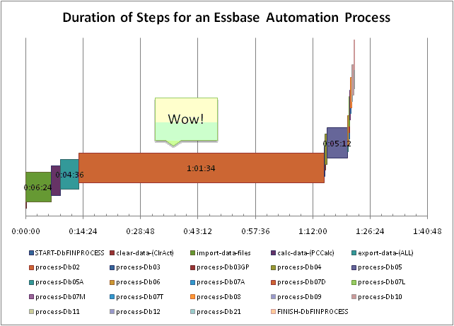
As part of looking at the bigger picture, I put together the following graph showing each step and how long it takes in this system that takes around an hour.  It’s not hard to tell that the majority of the time that it takes to run this job (the brownish bar that takes about an hour) is in one task!  And what is that task?  It’s a bunch of report scripts running on a staging database.  This is clearly an obvious place for me to look at ways of saving time.

The staging database is is a rather clever cube that is essentially used to scrub, aggregate, and associate raw account level data to some more meaningful dimensional combinations for all of the other databases.  Data comes in, it’s calculated, and it outputs a bunch of report scripts.  Fundamentally, the reason that this approach takes so much time is that there are two highly sparse dimension combinations with tens of thousands of members each, and the report script writer has to go through a ton of on-disk data in order to figure out what to write.  I could spend some time trying to optimize this process, in fact, I could probably play with some settings and get at least 20% improvement right now.

But, this is one of those times where it pays to stand back and look at what we’re trying to accomplish.  As it turns out, I actually have all of the infrastructure I need to accomplish this task, but it’s in a SQL database.  And, the task that is being performed is actually much more conducive to the way that a relational database works.  I’m still putting the finishing touches on this process, but it’s mostly complete as of right now, and the performance is amazing.  I can pump through the same amount of data in mere minutes now, with no loss of functionality.

My specific goal is to get this process that takes an hour or longer, to run in less than five minutes.  I chose this instead of “as fast as possible” because I wanted something concrete and attainable.  (My secret goal, just for kicks, is to get this all to run in under a minute).  Once the automation for the SQL staging is all in place, I will be going through all of the individual databases and tweaking any and all settings in order to shave their downtime as well.

Historically, not a lot of effort has gone into extensive profiling on these cubes, so as nerdy as it sounds, I’m actually very interested to see where else I can shave a few seconds off.  At first this will undoubtedly involve using more write threads in the dataload, rewriting the calc scripts to tighten them up from just their current CALC ALL, aligning the order of the data fields and rows with the dense/sparse-ness of the outlines and the outline order, choosing better cache settings that are customized for the size of the index and page files, and perhaps looking at benefits of zlib compression (theoretically more CPU time to compress/decompress, however, generally the CPUs on these servers are not slammed very hard, so if I can get the size of the physical page files down, I may be able to read it into memory faster).

So remember — you spend a lot of time doing calculations, but that might not alway be where the low hanging fruit is.  I cannot stress enough the importance of understanding where you spend your time, and using that as a basis for helping Essbase do its job faster.

There are numerous ASO cubes among my flock.  Usually the choice to use ASO was not arrived at lightly — it was/is for very specific technical reasons.  Typically, the main reason I have for using ASO is to get the fast data loads and the ability to load oodles of noodles… I mean data.  Yes, oodles of data.  The downsides (with version 7.x) is that I’m giving up calc scripts, incremental loading (although this has been somewhat addressed in later versions), native Dynamic Time Series, some flexiblity with my hierarchies, and I have to have just one database per application (you… uhh… were doing that already, right?).  Also, due to the sparsity of much of the data, trying to use BSO would result in a very unwieldy cube in this particular instance.

I have a set of four cubes that are all very similar, except for different Measures dimensions.  They range from 10,000 to 40,000 members.  This isn’t huge, but in conjunction with the sizes of the other dimensions, there is an incredible “maximum possible blocks” potential (sidenote for EAS: one of the most worthless pieces of information to know about your cube.  Really, why?).  The performance of these cubes is generally pretty acceptable (considering the amount of data), but occasionally user Excel queries (especially with attribute dimensions) really pound the server and take awhile to come back.  So I started looking into ways to squeeze out a little more performance.

Due to the nature of the aggregations in the cubes, they all have Dynamic hierarchies in the Accounts/Measures dimension.  This is due to using the minus (-) operator, some label only stuff, and shared members, all of which ASO is very particular with, especially in this version.  All of the other dimensions have Stored hiearchies or are set to Multiple Hierarchies (such as the MDX calcs in the Time dimension to get me some Year-To-Date members).

Actually, it turns out that all of the these cubes have Measures dimensions that make it prohibitively difficult to set Measures to Stored instead of Dynamic, except for one.  So, even though I would need to spin off a separate EIS metaoutline in order to build the dimension differently (these cubes are all generated from the same metaoutline but with different filters), it might be worth it if I can get some better performance on retrieves to this cube — particularly when the queries start to put some of the attribute dimensions or other MDX calcs into play.

What I need is some sort of method to test the performance of some typical retrieves against the two variants of the cube.  I setup one cube as normal, loaded it up with data, and materialized 1 gig worth of aggregations.  Prior to this I had also copied the cube within EAS, made the tweak to Measures to change it from Dynamic to Stored, loaded the data, did a gig of aggregations.  At this point I had two cubes with identical data but one with a Dynamic hierarchy (Measures with 10,000 or so members) and one with stored.  Time to compare.

I cooked up some report scripts, MaxL scripts, and some batch files.  The batch file loads a configuration file which specifies which database to hit and which report to run.  It then runs the report against the database, sets a timestamp before and after it runs, and dumps it all to a text file.  It’s not an exact science, but in theory it’ll give me somewhat of an idea as to whether making the hierarchy Stored is going to help my users’ retrieval operations.  And without further ado, here are the results:

Starting new process at Tue 01/20/2009 10:11:08.35		Time	Duration	Winner
	start-report_01-DB (Dynamic)	11:10.0
	finish-report_01-DB (Dynamic)	11:13.4	00:03.4
	start-report_01-DB (Stored)	11:14.6
	finish-report_01-DB (Stored)	11:21.4	00:06.8	Dynamic
	start-report_02-DB (Dynamic)	11:22.6
	finish-report_02-DB (Dynamic)	11:51.9	00:29.3
	start-report_02-DB (Stored)	11:53.0
	finish-report_02-DB (Stored)	12:00.0	00:07.0	Stored
	start-report_03-DB (Dynamic)	12:01.3
	finish-report_03-DB (Dynamic)	12:02.2	00:00.9
	start-report_03-DB (Stored)	12:03.9
	finish-report_03-DB (Stored)	12:42.1	00:38.2	Dynamic
	start-report_04-DB (Dynamic)	12:43.6
	finish-report_04-DB (Dynamic)	12:50.2	00:06.6
	start-report_04-DB (Stored)	12:51.3
	finish-report_04-DB (Stored)	14:26.4	01:35.1	Dynamic
	start-report_05-DB (Dynamic)	14:36.3
	finish-report_05-DB (Dynamic)	15:18.3	00:42.0
	start-report_05-DB (Stored)	15:19.6
	finish-report_05-DB (Stored)	17:32.0	02:12.4	Dynamic
Starting new process at Tue 01/20/2009 10:30:55.65
	start-report_01-DB (Dynamic)	30:57.5
	finish-report_01-DB (Dynamic)	30:59.9	00:02.4
	start-report_01-DB (Stored)	31:01.0
	finish-report_01-DB (Stored)	31:05.8	00:04.7	Dynamic
	start-report_02-DB (Dynamic)	31:07.7
	finish-report_02-DB (Dynamic)	31:40.8	00:33.1
	start-report_02-DB (Stored)	31:42.5
	finish-report_02-DB (Stored)	31:46.1	00:03.5	Stored
	start-report_03-DB (Dynamic)	31:50.4
	finish-report_03-DB (Dynamic)	31:51.0	00:00.6
	start-report_03-DB (Stored)	31:52.4
	finish-report_03-DB (Stored)	31:52.8	00:00.3	Tie
	start-report_04-DB (Dynamic)	31:54.0
	finish-report_04-DB (Dynamic)	32:06.3	00:12.3
	start-report_04-DB (Stored)	32:12.1
	finish-report_04-DB (Stored)	32:51.4	00:39.3	Dynamic
	start-report_05-DB (Dynamic)	32:55.5
	finish-report_05-DB (Dynamic)	33:38.1	00:42.6
	start-report_05-DB (Stored)	33:39.7
	finish-report_05-DB (Stored)	36:42.5	03:02.8	Dynamic

So, interestingly enough, the Dynamic dimension comes out on top, at least for most of the tests I wrote. There is one of the tests though (report_02) that seems to completely smoke the Dynamic hierarchy.  I wrote these report scripts kind of randomly, so I definitely need to do some more testing, but in the mean time I think I feel better about using a Dynamic hierarchy.  Since the ASO aggregation method for these cubes is simply to process aggregations until the database size is a certain multiple of it’s original size, one of the next steps I could look at for query optimization would be to enable query tracking, stuff the query statistics by running some reports, and then using those stats to design the aggregations.  In any case, I’m glad I am looking at some actual data rather than just blindly implementing a change and hoping for the best.

This isn’t to say that Dynamic is necessarily better than Stored or vice versa, however, I ran this very limited number of tests numerous times and got essentially the same results.  For the least part, this goes to show that there isn’t really a silver bullet for optimization and that experimentation is always a good way to go (except on your production servers, of course).  I am curious, however to go back and look at report_02 and see what it is about that particular report that is apparently so conducive to Stored hierarchies.

Sometimes you need to delete an Application but you can’t.  You still see it in Essbase Administration Services or even Application Manager (hey, there’s nothing wrong with still being on 6.5.x, if it ain’t broke…), but the app is broken or doesn’t exist.  The simplest cause of this is that someone [probably you] deleted the folder that contained the app, but you didn’t delete it through EAS.  And now, paradoxically enough, when you go in to EAS to delete the app, you can’t, because it can’t be started, because it doesn’t exist.  So essentially, the Essbase server tracks databases based not just on the existences of their folder, but also via some other means.

The easiest and most consistent method that I’ve come up with to kill the unruly app is this (assuming you have an extra Essbase server laying around):

1. On a separate Essbase server (your test server, for example), create an app of the same name, then create a database of the same name (you just have one database to an app, right?   No?  Well, go ahead and create the same-named databases — and shame on you, for cramming more than one database in an application).  If you already had a copy of the app/database on your test server, you can skip this part and just use the existing files.
2. Unload/stop the application you just created.
3. Stop the Essbase service on the server giving you troubles.
4. Copy the entire folder containing the new app to the proper location on the server that is messed up.  For example, if using Windows, if the name of your bad application is BadApp, right click on this folder from Windows Explorer and select Copy, then paste it into the app/folder on the server with the messed up app.  Use the appropriate cp -R command for Unix variants.
5. Restart the Essbase service, if necessary.
6. Start the App that was giving you problems.
7. Delete it (and make sure when you right click on Delete, you press it with authority.  You show that Essbase server who the boss is.)

This approach has always worked for me.  If you don’t have access to another Essbase server, you may be able to get away with following these steps, to an extent, using the same server —  I think I got that approach to work once but I really had to play with it and create the app with a different name, then go in and edit some of the files.

In any case, I hope this helps someone out there that is sick of looking at non-existant apps in their EAS view or just needs to fix something that went corrupt on them — so good luck y’all.

I got a question from a reader about how to do this.  Specifically, they were copying an application from one server to another and everything seemed to be going fine, except that there was no data in the resultant database on the target server.  The reason for this is that when you copy Essbase apps between servers, the data does not get copied.  If you copy the app on the server, it will copy the data.  So, how do we accomplish this?

For BSO cubes, the easiest option to do a cross server data copy is to copy the application by right-clicking on it, selecting Copy, then choosing the target server.  Then right-click on the database and select Export…. The export file will show up in your App folder were all of the Essbase applications are.  On your new (but empty) database that you just created from a copy, you can load this data.  If you have access to the File System locations, you can load the file across the servers, otherwise, you may have to copy/move the newly created export text file to a location that you can get to through the EAS Load file dialog box.  You don’t need any load rules since the data is already formatted in a way that is native to the application (just don’t make any changes to the outline before you import the data).

As I mentioned, when you copy an application to a new name on the same server, it will take the data with it — and anything in same folder as the app, for that matter.  So if you’re in the habit of storing gigs and gigs of text files in your database folder, get ready for a long wait as everything copies.  At least in version 7 of Essbase, copying huge applications is not a very graceful operation — it can stall the server while files are copying.  Even the best RAID setup can really take a pounding from all the reading and writing necessary to duplication an application.

For ASO databases, your options are a bit more limited since you can’t just do a database export.  You can still copy the applcation (and all it’s rule files and report scripts and such) across servers, though.  As I’m sure you’re aware by now, ASO databases can be quite a bit more fickle than BSO — and you’re quite used to ASO dumping all of your data when you even so much as look at the outline in the wrong way.  But part of the reason you are using ASO in the first place is for the fast loading times, even with massive datasets.  You can follow your same steps and load back data to ASO through EAS, or if you have setup your automation correctly, you can run your scripts and populate your new copy of the ASO application/database.

So, just what is this EIS thing?  You’ve heard about it, you know it has something to do with outlines, but you haven’t used it and you just don’t know where to start.  I understand.  I’ve been there.  I couldn’t really see an immediate payoff to using it, which kind of made getting all setup a little more daunting.  Please note that this article is written referring mostly to version 7 of EIS — I’m not sure what changes may have occurred since then.

Interestingly, my motivation for using EIS was a bit odd.  I was building some new cubes for the enterprise and they were in ASO for the first time.  The cubes were the evolution of a set of cubes that had been around in the company for a number of years, and the goal was to take what worked (and avoid what didn’t), and apply it for the entire organization.  Which is huge.  Hence the reason for ASO.  Along with learning all of the quirks that ASO brings to the table versus BSO, I also ran into another issue.  The original cubes, as part of their calculation method, would FIX on all of the accounts related to Gross Profit, flip the sign, and then roll up the whole cube.  The reason for this is that the GP accounts come in their “natural” accounting sign, so something like a sales account would be negative in the source database.  But since there are no calc scripts in ASO, I had to come up with another solution.  Well, it turns out that there’s this neat little feature on load rules that lets you flip the sign on a particular UDA.

Given that the Accounts dimension changes from period to period (and has  a bajillion members in it), it was necessary to come up with a mechanism to tag all of the appropriate accounts with the UDA I needed.  I got this working just fine with a load rule, ran it, and voila, I had a nice shiny UDA called “GP” on the members I needed.  I was feeling pretty pleased with myself… until the next time I ran the automation.  I ran it again and again for testing purposes.  And when I cracked open the outline again in EAS, I noticed that my members had about 20 copies of the “GP” UDA on them.

As it turns out, I believe this was a bonafide bug in Essbase 7.x that was fixed at some point — at the time I was writing the automation I believe my servers were 7.1.2.  But at the time we had no plans to put in the point upgrade, and not being the kind of guy that likes to wait around anyway, I decided to take the somewhat unconventional approach and just implement the entire thing in EIS.  So, you can honestly say that my entire reason for picking up EIS is because my UDAs were multiplying like tribbles on me, but that’s life, funny things like that happen.

So, getting back to the main idea here, what exactly is EIS?  In short, it’s a tool for creating outlines based on relational data.  It essentially takes the place of editing your outlines in EAS, using dimension build Load rules.  You can also load data through EIS (although I typically decline to do so and instead automate it with MaxL elsewhere).  And, unlike EAS with it’s oh-why-don’t-you-just-stab-me-in-the-eyes-already interface, EIS has a pretty slick interface.  In fact, the interface is so nice, it makes me just a little bit tingly on the inside… but then again that could just be related to my unnatural obsession with all things multi-dimensional.

Why use EIS?  Once you get good at it, and have some good upstream data to work with, you can crank out some outlines pretty fast.  You can also keep them updated very easily, by virtue of updating the source relational data that EIS reads.  I’m also completely and utterly sick of whipping up new load rules to update dimensions.  In the case of some of my attribute dimensions, I can’t even imagine the pain I would have to go through to implement the same functionality with a load rule.  EIS is also the tool you’ll need to use to link up to some drill-through data.

To get started with EIS, you need to make sure that EIS is installed on a server somewhere.  I just have mine running on the Essbase server itself and I find I am happy with this approach.  EIS will store all of it’s data in something referred to as the “metadata catalog,” which is just a SQL database that you’ll need to setup.  Oddly enough, when I started using EIS, I didn’t actually know I had a SQL server, but I figured there was one somewhere, so I started pinging things, and behold, I found a SQL box laying around (I guess the proper way of doing this would be to fill out a capital appropriations request for a server or something, but this makes a way better story).  It’s a SQL Server box with modest specs, but it gets the job done just fine.  It’s also the same server that I use to hold all of the relational data that I use for building outlines.

In a nutshell, you need to create a new database, then use one of the scripts that comes with EIS in order to populate the new database with some initial data.  This data is simply something that EIS will use under the hood and you won’t have to (and shouldn’t) edit the data by hand once you get it all loaded up.  After you have the shell of the metadata catalog setup, you will need to define some data sources from the EIS server to your relational data.  In my case, with Windows servers, this meant just setting up an ODBC connection on the Essbase server and pointing it to another new SQL database on the SQL server.

At this point, I would highly recommend following the EIS instructions and setting up the data they include for TBC (The Beverage Company).  Setting up this example means that you will be setup with the EIS Model for TBC, as well as a metaoutline for TBC.

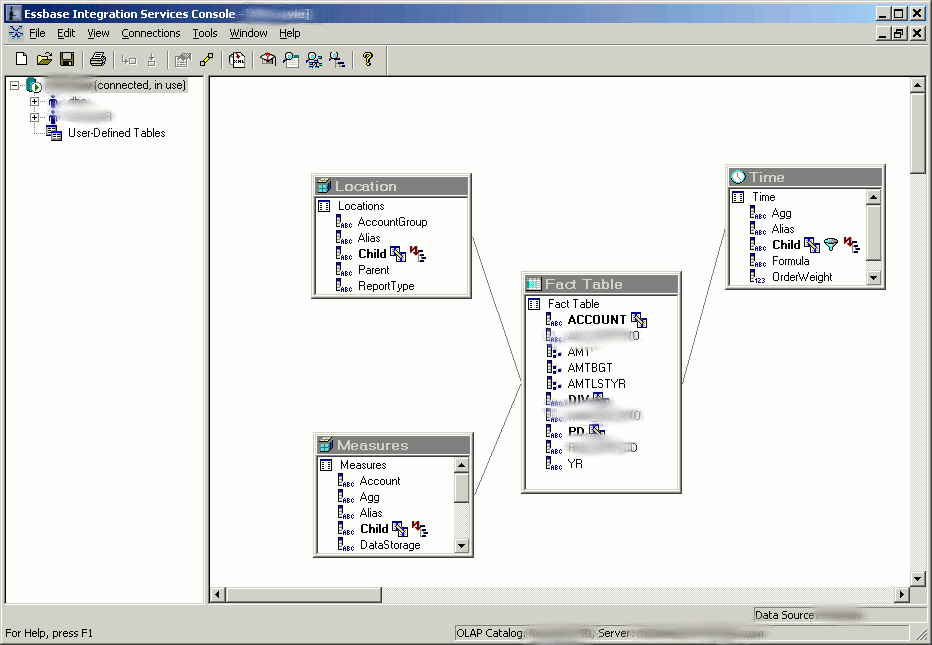
In EIS terminology, you create a model first, then a metaoutline.  A model is something you create in order to link together your SQL tables and tell EIS how they relate to each other.  At the center of this model you will have a Fact Table.  You can sort of think of the Fact Table as being similar in nature to the type of data that you would load to your Essbase cube with a normal load rule.  For example, if the rows in your data file had fields for the scenario, year, time period, location, department, measure, then a dollar amount or other figure, you can think of this as your fact table.  In this case, think of the different time periods for a moment.  In a typical periods/quarters/year setup, your text file would just have an 01 for period 01, an 02 for period 02, and so on.  Generally the source data wouldn’t make any sort of mention of the quarters, for example,  but EIS needs to know about this.  On the model, you would link the Period on the fact table to another table in your relational database that shows how to build the Time dimension based on that data.

The metaoutline has to be created after the model, because it is highly dependant on the way the model is setup.  In fact, when you create the metaoutline, you tell EIS which model to base it off of.  As the seasoned EIS veterans know about models and metaoutlines, once you commit to something in the model, you are basically married to it.  You can’t go around gutting the model too much unless you first make changes to your metaoutline(s).

If you’ve setup the model in a sane manner, you can then use the dimensions/tables you defined sort of as Lego blocks in your metaoutline, you can mix and match different dimensions and come up with a working outline.  You can even create arbitrary members in dimensions or completely new dimensions, if that’s what you need for that particular outline.  Try your best to keep it in the model though — it’ll usually pay off in the long run.

With the metaoutline properly defined, you can then load the members to a cube.  This is a straightforward process (assuming everything is setup correctly) where EIS will take your metaoutline, which is in turn based off your model, which is in turn based off your relational (SQL) data, and build a completely fresh outline for you.  Of course, this process can be automated (as with just about everything else).  If you’ve built everything correctly you can also load data through EIS too, although in practice I tend to find myself leaving that to an automation system, but it’s always good to know that your models are built properly.

The barriers to entry for setting up EIS can be daunting if you aren’t already using it.  You have to install it on a server, setup a SQL database for the metadata catalog, have some source data in SQL that you want to use to build/load outlines (which may require you to brush up on your SQL skills if you’re a bit rusty), and figure out how the tool works.  As always, learning from examples and experimenting on your own are very good ways to go — so if you can get the EIS demo app installed you should be able to see how things are put together.  The payoff though, for using EIS, can be immense.  You don’t have to mess around with all those dimension build load rules, you can spin up new outlines in a jiffy (without necessarily reinventing the wheel everytime), and girls think it’s pretty cool (and for all you female cube geeks out there, I’m sure the guys will be impressed too).

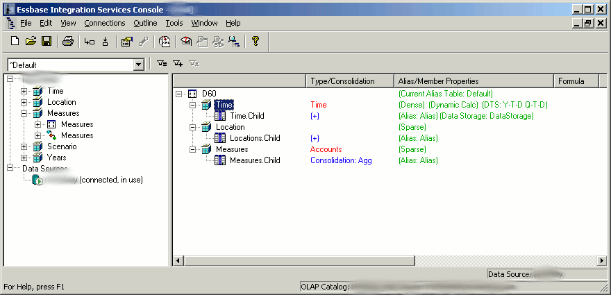
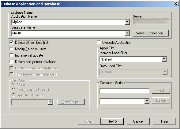
If you’re still curious about EIS (and who wouldn’t be?), feel free to drop me a line.  Also, if you’d like to see more articles about EIS, let me know and I get dig into some of the more complex stuff.  The screenshots below show some EIS screens — a model, a metaoutline, and building an outline from a metaoutline.   See in the model how the fact table is in the middle, with some other dimensions attached to it.  I blurred out some server information, but it doesn’t affect the purpose of the screenshot.