An Essbase Optimization Story

I got a call the other day from one of my fellow Essbase developers. One of the cubes in their budgeting system was taking a long time to finish calculations, whereas just days before the calculation time was just fine.  I have an almost unhealthy obsession with cube performance and optimization, so I jumped in to take a look.

The first thing I looked at (although not generally the first thing I look at) was the average cluster ratio.  The average cluster ratio is roughly analogous to the fragmentation of your hard drive: data gets added, removed, and the performance with regard to accessing that data is increasingly suboptimal.  Although the configuration of the sparse and dense dimensions in a BSO cube in theory dictates where data gets placed in the corresponding data files, quite often, for performance reasons, the data files will just grow to accomodate the new data instead of putting it where it “should” go.  A cluster ratio of 1.00 is optimal.  In this case, the database with performance issues was reporting a significantly lower cluster ratio.  So the first order of business was to export all of the data in the cube to a raw export file, clear the cube, then reimport.

This helped performance a little bit, but not much.  Something else needed to be done.  I checked out the index and page files in the cube directory to discover that the index files were almost four gigabytes, with about 20 gigabytes of page files.  This size of data isn’t inherently difficult to work with, but it does warrant a look into the dense and sparse dimension settings,  the calc script that is having issues, and trying to understand the way in which the database data is being used.

The database is a six dimension cube with the following dimensions: Scenario, Years, Time, Location, Customer, Commodities.  Time and Scenario are marked as dense.  I can live with Time being dense, especially since it’s just periods rolling to quarters rolling to a fiscal year (with non-Level 0 members tagged as Dynamic Calc), but the dense Scenario dimension didn’t quit jive with me.  In this particular database, it turns out that the reason for the block explosion and subsequent poor calc performance is that users and loading in tons of data to the Forecast member in Scenario.  Scenario also has four other dense members.  In addition to the cube being to to create blocks new blocks on equations, the size of the page files was blowing out with all of the data being sent in.

The first thing that jumps out at me is that even though all of this data is being loaded to the Forecast member, we’re taking a hit on storage because the dense data blocks are being allocated for the other four members in Scenario that are very sparingly utilized.  Surely there is a better candidate for a dense dimension?  You betcha.  Given the sparse nature of the database, most of the other dimensions aren’t really good candidates for dense because of all the interdimensional irrelevance that it would incur, however, the Years dimension is a good candidate because the Forecast data being loaded in is being loaded in for a particular year and all periods.  Perfect.

Given that there are not a significant number of calc, report, and load scripts in this database, it is relatively safe to change the dimensional configuration here.  This isn’t always necessarily the case and changing dense/sparse settings could very easily deoptimize the performace of calc, load, and report scripts, not to mention adversely affecting other numerous aspects of the database.

And of course, this was all tested on the test server before loading to production.  The process was fairly straightforward.  I cleared the database again, and loaded the export file.  Since export files are sensitive to the dense/sparse settings in the database, I did this so I could restructure the database with the new settings and have Essbase do the work for me instead of having to load the data from somewhere else.  I also made sure to do this before doing a calculation on the database so there would be less data to restructure.  After the data loaded in, I changed the dense and sparse settings to set Years to dense and Scenario to sparse.  After the restructure, database statistics were looking fairly good, but I didn’t want to get my hopes up.

Clearly one of the issues with this database was that the calculation script that was taking too long had to span through 20 gigabytes of page files in order to do what it needed to do.  Generally my databases are set to bitmap encoding as the compression scheme (because in most cases it is “good enough”), but I decided to go with zlib compression instead.  Although technically speaking, zlib is more computationally intensive to compress and uncompress, because our servers’ CPUs aren’t generally getting hammered, I decided that I would rather hit the CPUs a little harder if it meant that I could read the data off the disk a little faster (even though it will still uncompress in memory to the same amount as bitmap encoding or any other compression scheme).  Conversely, the stronger compression will mean less data is also written to the disk.

I then had to do some tweaking to the calc script to align it with the next dense and sparse settings.  This was fairly easy.  As with most calc script optimization, this involved changing the FIX statements and CALC DIM statements so that I was fixing on sparse dimensions and doing as much calculating within the dense data block as possible.  Remember, you are always trying to help Essbase do its job and give it hints as to how it can do things more optimally.  In this case, we are trying to minimize the amount of data that must be scanned through.  By calculating within the dense blocks, we are doing all of the work in one place that we can, then moving on to the next area.  For good measure, I also added a SET command to utilize the server’s higher calc lock block setting (see your technical reference for more details).

I fired off the calculation and checked out the results.  The calculation’s first pass took about 20 minutes (a lot of blocks were being created the first time around).  After this pass was done, I checked out the index and page files.   The index file seemed to be holding steady at about 300 megabytes — quite an improvement from four gigs!  The page file was now about 700 megabytes.  Given this new page file size, I decided to set the index cache to 512 megabytes.  Although this will eat 512 megabytes directly out of memory on the server, we have decided to allocate more memory for this app until forecasts are done, then we can pull back on the amount of memory it gets.  But for now, with enough memory to hold the entire index at one time, calculations and other operations will be much faster.

At the time of this writing, the database calculation that was the original problem is still holding steady at about 10 minutes to calculate.  The page and index files have grown a bit but still appear to be holding steady, and the database statistics indicate a pretty good block density as well.  Not a bad bit of optimization — a twentyfold decrease in size on disk, and a calculation that comes back in minutes rather than never.

Like I said, I love performance optimization, and as I’ve said before, Essbase is a bit of an art and a science.  The art part is comprehensively understanding how things work and how they are meant to work, then using that information to make the right technical tradeoffs, then putting the changes into the system, keeping in mind that you are simply trying to give “hints” to the system to help it do its job a little better or faster.
Essbase Performance Optimization: it’s not just the calc script

Here’s a quick post that is a bit of a precursor to some of my more in-depth performance analysis articles that will be coming out in the future.  One of my automation systems takes a bit over an hour to run.  There are a lot of people I know that need to squeeze performance out of their systems and immediately look to their calc scripts.  Yes, calc time can be a large part of your downtime, as can data loads, reports, and other activities.  But I always stress that it is useful and important to understand your systems in their entirety.

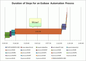
As part of looking at the bigger picture, I put together the following graph showing each step and how long it takes in this system that takes around an hour.  It’s not hard to tell that the majority of the time that it takes to run this job (the brownish bar that takes about an hour) is in one task!  And what is that task?  It’s a bunch of report scripts running on a staging database.  This is clearly an obvious place for me to look at ways of saving time.

Duration of Steps for an Essbase Automation Process

Duration of Steps for an Essbase Automation Process

The staging database is is a rather clever cube that is essentially used to scrub, aggregate, and associate raw account level data to some more meaningful dimensional combinations for all of the other databases.  Data comes in, it’s calculated, and it outputs a bunch of report scripts.  Fundamentally, the reason that this approach takes so much time is that there are two highly sparse dimension combinations with tens of thousands of members each, and the report script writer has to go through a ton of on-disk data in order to figure out what to write.  I could spend some time trying to optimize this process, in fact, I could probably play with some settings and get at least 20% improvement right now.

But, this is one of those times where it pays to stand back and look at what we’re trying to accomplish.  As it turns out, I actually have all of the infrastructure I need to accomplish this task, but it’s in a SQL database.  And, the task that is being performed is actually much more conducive to the way that a relational database works.  I’m still putting the finishing touches on this process, but it’s mostly complete as of right now, and the performance is amazing.  I can pump through the same amount of data in mere minutes now, with no loss of functionality.

My specific goal is to get this process that takes an hour or longer, to run in less than five minutes.  I chose this instead of “as fast as possible” because I wanted something concrete and attainable.  (My secret goal, just for kicks, is to get this all to run in under a minute).  Once the automation for the SQL staging is all in place, I will be going through all of the individual databases and tweaking any and all settings in order to shave their downtime as well.

Historically, not a lot of effort has gone into extensive profiling on these cubes, so as nerdy as it sounds, I’m actually very interested to see where else I can shave a few seconds off.  At first this will undoubtedly involve using more write threads in the dataload, rewriting the calc scripts to tighten them up from just their current CALC ALL, aligning the order of the data fields and rows with the dense/sparse-ness of the outlines and the outline order, choosing better cache settings that are customized for the size of the index and page files, and perhaps looking at benefits of zlib compression (theoretically more CPU time to compress/decompress, however, generally the CPUs on these servers are not slammed very hard, so if I can get the size of the physical page files down, I may be able to read it into memory faster).

So remember — you spend a lot of time doing calculations, but that might not alway be where the low hanging fruit is.  I cannot stress enough the importance of understanding where you spend your time, and using that as a basis for helping Essbase do its job faster.

MaxL Essbase automation patterns: moving data from one cube to another

A very common task for Essbase automation is to move data from one cube to another.  There are a number of reasons you may want or need to do this.  One, you may have a cube that has detailed data and another cube with higher level data, and you want to move the sums or other calculations from one to the other.  You may accept budget inputs in one cube but need to push them over to another cube.  You may need to move data from a “current year” cube to a “prior year” cube (a data export or cube copy may be more appropriate, but that’s another topic).  In any case, there are many reasons.

For the purposes of our discussion, the Source cube is the cube with the data already in it, and the Target cube is the cube that is to be loaded with data from the source cube.  There is a simple automation strategy at the heart of all these tasks:

  1. Calculate the source cube (if needed)
  2. Run a Report script on the source cube, outputting to a file
  3. Load the output from the report script to the target cube with a load rule
  4. Calculate the target cube

This can be done by hand, of course (through EAS), or you can do what the rest of us lazy cube monkeys do, and automate it.  First of all, let’s take a look at a hypothetical setup:

We will have an application/database called Source.Foo which represents our source cube.  It will have dimensions and members as follows:

  • Location: North, East, South, West
  • Time: January, February, …, November, December
  • Measures: Sales, LaborHours, LaborWages

As you can see, this is a very simple outline.  For the sake of simplicity I have not included any rollups, like having “Q1/1st Quarter” for January, February, and March.  For our purposes, the target cube, Target.Bar, has an outline as follows:

  • Scenario: Actual, Budget, Forecast
  • Time: February, …, November, December
  • Measures: Sales, LaborHours, LaborWages

These outlines are similar but different.  This cube has a Scenario dimension with Actual, Budget, and Forecast (whereas in the source cube, since it is for budgeting only, everything is assumed to be Budget).  Also note that Target.Bar does not have a Location dimension, instead, this cube only concerns itself with totals for all regions.  Looking back at our original thoughts on automation, in order for us to move the data from Source.Foo to Target.Bar, we need to calculate it (to roll-up all of the data for the Locations), run a report script that will output the data how we need it for Target.Bar, use a load rule on Target.Bar to load the data, and then calculate Target.Bar.  Of course, business needs will affect the exact implementation of this operation, such as the timing, the calculation to use, and other complexities that may arise.  You may actually have two cubes that don’t have a lot in common (dimensionally speaking), in which case, your load rule might need to really jump through some hoops.

We’ll keep this example really simple though.  We’ll also assume that the automation is being run from a Windows server, so we have a batch file to kick things off:

cd /d %~dp0
essmsh ExportAndLoadBudgetData.msh

I use the cd /d %~dp0 on some of my systems as a shortcut to switch the to current directory, since the particular automation tool installed does not set the home directory of the file to the current working directory.  Then we invoke the MaxL shell (essmsh, which is in the PATH) and run ExportAndLoadBudgetData.msh.  I enjoy giving my automation files unnecessarily long filenames.  It makes me feel smarter.

As you may have seen from an earlier post, I like to modularize my MaxL scripts to hide/centralize configuration settings, but again, for the sake of simplicity, this example will forgo that.  Here is what ExportAndLoadBudgetData.msh could look like:

/* Copies data from the Budget cube (Source.Foo) to the Budget Scenario
   of Target.Bar */
/* your very standard login sequence here */
login AdminUser identified by AdminPw on EssbaseServer;
/* at this point you may want to turn spooling on (omitted here) */

/* disable connections to the application -- this is optional */
alter application Source disable connects;

/* PrepExp is a Calc script that lives in Source.Foo and for the purposes
   of this example, all it does is makes sure that the aggregations that are
   to be exported in the following report script are ready. This may not be
   necessary and it may be as simple as a CALC ALL; */

execute calculation Source.Foo.PrepExp;

/* Budget is the name of the report script that runs on Source.Foo and outputs a
   text file that is to be read by Target.Bar's LoadBud rules file */

export database Source.Foo
    using report_file 'Budget'
    to data_file 'foo.txt';

/* enable connections, if they were disabled above */
alter application Source enable connects;
/* again, technically this is optional but you'll probably want it */
alter application Target disable connects;

/* this may not be necessary but the purpose of the script is to clear out
   the budget data, under the assumption that we are completely reloading the
   data that is contained in the report script output */

execute calculation Target.Bar.ClearBud;

/* now we import the data from the foo.txt file created earlier. Errors
   (rejected records) will be sent to errors.txt */

import database Target.Bar data
    from data_file 'foo.txt'
    using rules_file 'LoadBud'
    on error write to 'errors.txt';

/* calculate the new data (may not be necessary depending on what the input
   format is, but in this example it's necessary */

execute calculation Target.Bar.CalcAll;

/* enable connections if disabled earlier */
alter application Target enable connects;
/* boilerplate cleanup. Turn off spooling if turned on earlier */

logoff;
exit;

At this point , if we don’t have them already, we would need to go design the aggregation calc script for Source.Foo (PrepExp.csc), the report script for Source.Foo (Budget.rep), the clearing calc script on Target.Bar (ClearBud.csc), the load rule on Target.Bar (LoadBud.rul), and the final rollup calc script (CalcAll.csc).  Some of these may be omitted if they are not necessary for the particular process (you may opt to use the default calc script, may not need some of the aggregations, etc).

For our purposes we will just say that the PrepExp and CalcAll calc scripts are just a CALC ALL or the default calc.  You may want a “tighter” calc script, that is, you may want to design the calc script to run faster by way of helping Essbase understand what you need to calculate and in what order.

What does the report script look like?  We just need something to take the data in the cube and dump it to a raw text file.

<ROW ("Time", "Measures")

{ROWREPEAT}
{SUPHEADING}
{SUPMISSINGROWS}
{SUPZEROROWS}
{SUPCOMMAS}
{NOINDENTGEN}
{SUPFEED}
{DECIMAL 2}

<DIMBOTTOM "Time"
<DIMBOTTOM "Measures"
"Location"
!

Most of the commands here should be pretty self explanatory.  If the syntax looks a little different than you’re used to, it’s probably because you can also jam all of the tokens in one line if you want like {ROWREPEAT SUPHEADING} but historically I’ve had them one to a line.  If there were more dimensions that we needed to represent, we’d put thetm on the <ROW line.  As per the DBAG, we know that the various tokens in between {}’s format the data somehow — we don’t need headings, missing rows, rows that are zero (although there are certainly cases where you might want to carry zeros over), no indentation, and numbers will have two decimal places (instead of some long scientific notation). Also, I have opted to repeat row headings (just like you can repeat row heading in Excel) for the sake of simplicity, however, as another optimization tip, this isn’t necessary either — it just makes our lives easier in terms of viewing the text file and loading it to a SQL database or such.

As I mentioned earlier, we didn’t have rollups such as different quarters in our Time dimension.  That’s why we’re able to get away with using <DIMBOTTOM, but if we wanted just the Level 0 members (the months, in this case), we could use the appropriate report script.  Lastly, from the Location dimension we are taking use the Location member (whereas <DIMBOTTOM “Time” tells Essbase to give us all the members to the bottom of the Time dimension, simply specifying a member or members from the dimension will give us those members), the parent to the different regions.  “Location” will not actually be written in the output of the report script because we don’t need it — the outline of Target.Bar does not have a location dimension since it’s implied that it represents all locations.

The output of the report script will look similar to the following:

January Sales 234.53
January LaborHours 35.23
February Sales 532.35

From here it is a simple matter of designing the load rule to parse the text file.  In this case, the rule file is part of Target.Bar and is called LoadBud.  If we’ve designed the report script ahead of time and run it to get some output, we can then go design the load rule.  When the load rule is done, we should be able to run the script (and schedule it in our job scheduling software) to carry out the task in a consistent and automated manner.

As an advanced topic, there are several performance considerations that can come into play here.  I already alluded to the fact that we may want to tighten up the calc scripts in order to make things faster.  In small cubes this may not be worth the effort (and often isn’t), but as we have more and more data, designing the calc properly (and basing it off of good dense/sparse choices) is critical.  Similarly, the performance of the report script is also subject to the dense/sparse settings, the order of the output, and other configuration settings in the app and database.  In general, what you are always trying to do (performance wise) is to help the Essbase engine do it’s job better — you do this by making the tasks you want to perform more conducive to the way that Essbase processes data.  In other words, the more closely you can align your data processing to the under-the-hood mechanisms of how Essbase stores and manipulates your data, the better off you’ll be.  Lastly, the load rule on the Target database, and the dense/sparse configurations of the Target database, will impact the data load performance.  You may not and probably will not be able to always optimize everything all at once — it’s a balancing act — since a good setting for a report script may result in suboptimal calculation process.  But don’t let this scare you — try to just get it to work first and then go in and understand where the bottlenecks may be.

As always, check the DBAG for more information, it has lots of good stuff in it.  And of course, try experimenting on your own, it’s fun, and the harder you have to work for knowledge, the more likely you are to retain it.  Good luck out there!

Optimizing Essbase Automation Jobs (for fun and profit!) – Part 1

I freely submit that I am a complete geek.  But it’s okay, because I have come to accept and embrace that inner geek.  Anyway… Many organizations run jobs to perform a task as certain intervals.  Your job as a good Essbase/Hyperion administrator is to be lazy — that is, make the computers do the boring stuff, while you get to do the fun stuff, like thinking.  What we end up doing is setting up batch and script files that do all of the things in a particular sequence that we might do by hand.  So instead of logging in, copying a data file, clearing a cube, running a calc, loading some data, running another calc, and all that other stuff, we do this automatically.

After a while, you get a feel for how long a certain job takes.  The job that loads last week’s sales might take about an hour to run.  The job to completely restate the database for the entire fiscal year might take six hours to run.  This probably also becomes painfully obvious when it turns out that the job didn’t run correctly, and now you need to run it again (and keep those users happy).  I am all about jobs running as fast as they can.  This is useful on a few different levels.  First and probably foremost, it finishes faster, which is nice, especially for those times when the sooner you have data the better.  It’s also nice when you need to re-run things.  It can also open up some new possibilities to use the tool in ways you didn’t think or know you could — such as during the business week, getting live updates of data.

Typically there are a few big time-killers in an automated process.  These are the data loads, calculations, and reports that are run.  There are also some others, such as calling out to a SQL server to do some stuff, restructuring outlines, pulling tons of data off the WAN, and all that.  You can always go through your database logs to see how long a particular calculation took, but this is a bit tedious.  Besides, if you’re like me, then you want to look under EVERY single nook and cranny for places to save a little time.  To borrow an a saying from the race car world, instead of finding one place to shave off 100 pounds, we can find 100 places to shave off one pound.  In practice, of course, some of these places you can’t cut anything from, but some of them you can cut down quite a bit.

The first, and probably most important step to take is to simply understand where you are spending your processing time.  This will give you a better window into where you spend time, rather than just a few things in the normal Essbase logs.  There are numerous ways you can do this.  But, if you know me at all by now, you know that I like to do things on the cheap, and make them dead-simple.  That being said, the following posts will be based around Windows batch file automation, but the concepts are easily portable to any other platform.

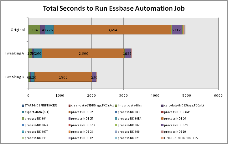
First of all, take a look at the below graph:

Total Seconds to Run Essbase Automation Job

Total Seconds to Run Essbase Automation Job

What you’re looking at is a graph that has been created in Excel, based on data in a text file that was generated as a result of a profiling process.  The steps are as granular as we want them to be.  In other words, if we simply want to clump together a bunch of jobs that all run really fast, then we can do that.  Similarly, if we want to break down a single job that seems to take a relatively long amount of time, we can do that too.  Each segment in the starcked bar chart is based on the number of seconds that the particular step took.  We can see that in the original (pre-optimization) scenario, the orangey-brown step takes up a pretty considerable amount of the overall processing time.  After some tweaking, we were able to dramatically slash the amount of time that it took to run the whole job.  And, in the third bar, after yet more tweaking, we were able to slash the overall processing time quite a bit again.

The important thing here is that we are now starting to build an understanding of exactly where we are spending our time — and we can therefore prioritize where we want to attempt to reduce that time.  My next post will detail a sample mechanism for getting this kind of raw data into a file, and the next few posts after those will start to dig in to where and how time was shaved off due to better outline, system, and other settings and changes.  Happy profiling!

Jason’s Top 10 Essbase Data Load Optimization Tips

I received an email today from someone looking to speed up their data loads, specifically their ASO data loads that seem to be taking too long.  This is, of course, an important topic for many Essbase cube wranglers.  I would be willing to bet that many people spend more time optimizing calcs and may even neglect profiling their performance on data loads.  You might be surprised just how long your automation spends doing a data load.  That being said, there are several different scenarios you may find yourself in and different places to optimize.  Of course there are more items that can go on this list, but here are the big ones off the top of my head.  In other words, if I was tasked with improving my data load speed, here’s what I would look at:

  1. Do you need to load the data in the first place? I know this seems a bit rudimentary, but if you are loading data that you don’t even need (and can possibly help it), then don’t waste your time on it.
  2. Use the fastest connection. Architecturally you may simply have to load data one way or another (from a text file, from a SQL server, off the SAN, etc), but, hands down the fastest data loads I’ve seen (short of trying to load from a RAMdisk, although I’m dying to try it) are from different physical hard drives attached to the Essbase server.  With a good RAID setup the performance is still quite good if you are loading text files from the Essbase server.  If you are loading your records from an RDBMS across the WAN, you might be killing your performance due to network bottlebecks.  Another option is to put the RDBMS on the same box as Essbase.  I know many people do this, but personally I am not a huge fan of this option.  My Essbase servers tend to have plenty enough to do without having SQL software on the box to worry about.  Additionally, we license SQL by the CPU, and since my Essbase servers are all quad-proc and the SQL servers are getting by just fine with dual-proc, the cost to license it for two more CPUs is quite significant — particularly when all of the other optimization methods are essentially ‘free’.
  3. If loading from a SQL RDBMS: your bottleneck may very well be the network speed here.  If you can, make sure your Essbase server is on the same LAN as the SQL server, with the fastest possible connections (Gigabit or better).  If you are loading from a SQL table and using the WHERE clause in your load rule, or you are loading from a SQL view, make sure you have good indexes setup in SQL.  This can make a HUGE difference if you are loading just the records from Period 08 and you have an index, versus making the SQL server scan the entire table.  If performance is extremely critical see if you can pre-stage text files on the Essbase server (like tip #2).  If loading to BSO, order the rows to match your dense/sparse settings and the order of the outline (basically, you are trying to give Essbase a hand and load up a whole dense datablock in as few passes as possible).
  4. Do as little work as possible in the load rule.  The cost of doing text replacements, column swaps, accept/reject rules, and all that stuff can really add up.  If you can do this elsewhere then do it there (e.g., in a SQL view or having your ETL software prep it for you in the format you need).
  5. Tweak your settings. The Essbase.cfg has some black magic stuff in it.  Try the DLTHREADSWRITE parameter (check the DBAG for details) to see if you can throw some threads at the problem.  Watch your performance on the server — slamming all the CPUs may cause performance for other users to decrease.
  6. (BSO) Sort the data.  Try to give Essbase a a hand.  If your records are sorted such that Essbase is looking at the fewest blocks at a time, and reading the items in the same order as the outline, you’ll reduce the punishment to Essbase and help it load records faster.
  7. Outline optimization.  This one, of course, applies to just about everything you do in Essbase.  Smaller datablocks are your friends — in the sense that if you are committed to your dense/sparse settings, see if you can lighten up the dense blocks with some strategic dynamic calcs and labels.  For instance, my Time dimension is usually Time –> Quarters –> Periods and nine times out of ten, when Time is dense, the Quarters and Time members are dynamic calc instead of stored.  Of course, there may be numerous other reasons that the dense/sparse settings are what they are (calc performance, retrieve performance, etc), so don’t go making changes without understanding them.
  8. Load and Swap. You may find it useful to load up a cube separate from the production cube, then implement MaxL to drop it on top of the production cube (all on the same server of course).  This way you do all of the hard work in one and when it’s ready you can just pop it in place.  I think this works better in theory than in practice, at least for me.  I initially tried this with some very large ASO cubes, and although the performance wasn’t terrible, at least with version 7.1.x of Essbase, the swap process (the MaxL was a “create or replace” command) was not very graceful — it would shake the server to its knees during the swap process.  I eventually dropped this method in favor of using all the other points to optimize and make the down time even smaller.
  9. Use your own load rules instead of EIS. Out of convenience, and particularly on small cubes, I will load data with EIS.  However, you are going to see better performance when you use your own load rules and optimize them.  Besides, you probably already did it this way since you are concerned about performance, and this is probably in an automation script anyway.
  10. Reduce the size of the data members.  Any time your bottleneck is the speed of the transmission of information, try to cut it down (particuarly for SQL loads across the LAN).  For example, don’t have the field be “Period 01” if you can use “P01” instead.  Use “08” instead of “Yr2008”.  Try to balance this with how much work your load rule is doing (Tip #4).

As always, experiment!  Try different combinations to see what works and what doesn’t.  Remember that for squeezing out that extra bit of performace, you are trying to help Essbase do its job better.  Always remember that dimensions can be and probably are (on cubes you didn’t build) setup how they are setup for a reason — i.e., you might have worse load time but the benefit is faster calc or retrieve time.  If you have your own tips please let me know!