jason w. jones

software from the trenches

Essbase, the economy and thoughts from the last ODTUG

I was going through some papers today and I happened to come across a sheet of my notes that I jotted down while I was at ODTUG in New Orleans last year (the best Hyperion conference around, seriously).  Coincidentally, earlier in the day I also had a conversation with a colleague of mine who works at a sizable company that does not significantly utilize BI/EPM.  She said they had looked at some options, including Essbase, but at the end of the day that just couldn’t justify the cost to get up and running — especially in “this economy” where everything else is being cut back, scaled down, or eliminated.

My question to her was this: how can you afford not to?  I noticed that many of the points I had taken away from various presenters and people I talked to at the conference wove in perfectly with this company’s predicament.  In the next paragraph I’ve italicized my original notes and added some context .  So, is investing in Essbase worth the money, especially in this economy where each dollar is even more critical than before?  Yes.

There are countless ways for companies to improve their business.  Essbase is just one of the many tools that companies can put in their toolbox.  Many companies have built up vast warehouses of data over the years, but aren’t leveraging it.  Even if your company is already using Hyperion, Oracle, or other software to analyze data, there is probably a lot of room to expand the usage.  You know why?  Because companies under-utilize the tools that they have. It takes mastery to unlock the full potential of a tool.

Essbase is worth its weight in gold, because when it’s implemented properly, it can tell you a lot about your business.  Specifically, it can tell you where you are losing money. Tools such as Essbase and associated functionality are about doing business better, not just doing business. It is a very adept tool for painting a picture of alternative futures — because this is where the improvements happen.

I was pretty happy to come across a sheet of my notes that I had tucked away, because many of things I saw and heard at the conference were so poignant — and directly applicable to the real world.  It’s nice to step back for a moment from being so engrossed in the technical aspects of the technology and think for a moment about the bigger picture and why I do what I do.  I enjoy what I do because I have powerful and flexible tools in my toolbox that are the best in the business.  I do my best to put them to good use and this allows me to make a positive impact on the business, help people in the company (who in turn help customers — and the stockholders), and enjoy the recognition that comes from being good at my chosen endeavors.  And to top it all off, it’s just plain fun to be a cube monkey.

MaxL Essbase automation patterns: moving data from one cube to another

A very common task for Essbase automation is to move data from one cube to another.  There are a number of reasons you may want or need to do this.  One, you may have a cube that has detailed data and another cube with higher level data, and you want to move the sums or other calculations from one to the other.  You may accept budget inputs in one cube but need to push them over to another cube.  You may need to move data from a “current year” cube to a “prior year” cube (a data export or cube copy may be more appropriate, but that’s another topic).  In any case, there are many reasons.

For the purposes of our discussion, the Source cube is the cube with the data already in it, and the Target cube is the cube that is to be loaded with data from the source cube.  There is a simple automation strategy at the heart of all these tasks:

  1. Calculate the source cube (if needed)
  2. Run a Report script on the source cube, outputting to a file
  3. Load the output from the report script to the target cube with a load rule
  4. Calculate the target cube

This can be done by hand, of course (through EAS), or you can do what the rest of us lazy cube monkeys do, and automate it.  First of all, let’s take a look at a hypothetical setup:

We will have an application/database called Source.Foo which represents our source cube.  It will have dimensions and members as follows:

  • Location: North, East, South, West
  • Time: January, February, …, November, December
  • Measures: Sales, LaborHours, LaborWages

As you can see, this is a very simple outline.  For the sake of simplicity I have not included any rollups, like having “Q1/1st Quarter” for January, February, and March.  For our purposes, the target cube, Target.Bar, has an outline as follows:

  • Scenario: Actual, Budget, Forecast
  • Time: February, …, November, December
  • Measures: Sales, LaborHours, LaborWages

These outlines are similar but different.  This cube has a Scenario dimension with Actual, Budget, and Forecast (whereas in the source cube, since it is for budgeting only, everything is assumed to be Budget).  Also note that Target.Bar does not have a Location dimension, instead, this cube only concerns itself with totals for all regions.  Looking back at our original thoughts on automation, in order for us to move the data from Source.Foo to Target.Bar, we need to calculate it (to roll-up all of the data for the Locations), run a report script that will output the data how we need it for Target.Bar, use a load rule on Target.Bar to load the data, and then calculate Target.Bar.  Of course, business needs will affect the exact implementation of this operation, such as the timing, the calculation to use, and other complexities that may arise.  You may actually have two cubes that don’t have a lot in common (dimensionally speaking), in which case, your load rule might need to really jump through some hoops.

We’ll keep this example really simple though.  We’ll also assume that the automation is being run from a Windows server, so we have a batch file to kick things off:

cd /d %~dp0
essmsh ExportAndLoadBudgetData.msh

I use the cd /d %~dp0 on some of my systems as a shortcut to switch the to current directory, since the particular automation tool installed does not set the home directory of the file to the current working directory.  Then we invoke the MaxL shell (essmsh, which is in the PATH) and run ExportAndLoadBudgetData.msh.  I enjoy giving my automation files unnecessarily long filenames.  It makes me feel smarter.

As you may have seen from an earlier post, I like to modularize my MaxL scripts to hide/centralize configuration settings, but again, for the sake of simplicity, this example will forgo that.  Here is what ExportAndLoadBudgetData.msh could look like:

/* Copies data from the Budget cube (Source.Foo) to the Budget Scenario
   of Target.Bar */
/* your very standard login sequence here */
login AdminUser identified by AdminPw on EssbaseServer;
/* at this point you may want to turn spooling on (omitted here) */

/* disable connections to the application -- this is optional */
alter application Source disable connects;

/* PrepExp is a Calc script that lives in Source.Foo and for the purposes
   of this example, all it does is makes sure that the aggregations that are
   to be exported in the following report script are ready. This may not be
   necessary and it may be as simple as a CALC ALL; */

execute calculation Source.Foo.PrepExp;

/* Budget is the name of the report script that runs on Source.Foo and outputs a
   text file that is to be read by Target.Bar's LoadBud rules file */

export database Source.Foo
    using report_file 'Budget'
    to data_file 'foo.txt';

/* enable connections, if they were disabled above */
alter application Source enable connects;
/* again, technically this is optional but you'll probably want it */
alter application Target disable connects;

/* this may not be necessary but the purpose of the script is to clear out
   the budget data, under the assumption that we are completely reloading the
   data that is contained in the report script output */

execute calculation Target.Bar.ClearBud;

/* now we import the data from the foo.txt file created earlier. Errors
   (rejected records) will be sent to errors.txt */

import database Target.Bar data
    from data_file 'foo.txt'
    using rules_file 'LoadBud'
    on error write to 'errors.txt';

/* calculate the new data (may not be necessary depending on what the input
   format is, but in this example it's necessary */

execute calculation Target.Bar.CalcAll;

/* enable connections if disabled earlier */
alter application Target enable connects;
/* boilerplate cleanup. Turn off spooling if turned on earlier */

logoff;
exit;

At this point , if we don’t have them already, we would need to go design the aggregation calc script for Source.Foo (PrepExp.csc), the report script for Source.Foo (Budget.rep), the clearing calc script on Target.Bar (ClearBud.csc), the load rule on Target.Bar (LoadBud.rul), and the final rollup calc script (CalcAll.csc).  Some of these may be omitted if they are not necessary for the particular process (you may opt to use the default calc script, may not need some of the aggregations, etc).

For our purposes we will just say that the PrepExp and CalcAll calc scripts are just a CALC ALL or the default calc.  You may want a “tighter” calc script, that is, you may want to design the calc script to run faster by way of helping Essbase understand what you need to calculate and in what order.

What does the report script look like?  We just need something to take the data in the cube and dump it to a raw text file.

<ROW ("Time", "Measures")

{ROWREPEAT}
{SUPHEADING}
{SUPMISSINGROWS}
{SUPZEROROWS}
{SUPCOMMAS}
{NOINDENTGEN}
{SUPFEED}
{DECIMAL 2}

<DIMBOTTOM "Time"
<DIMBOTTOM "Measures"
"Location"
!

Most of the commands here should be pretty self explanatory.  If the syntax looks a little different than you’re used to, it’s probably because you can also jam all of the tokens in one line if you want like {ROWREPEAT SUPHEADING} but historically I’ve had them one to a line.  If there were more dimensions that we needed to represent, we’d put thetm on the <ROW line.  As per the DBAG, we know that the various tokens in between {}’s format the data somehow — we don’t need headings, missing rows, rows that are zero (although there are certainly cases where you might want to carry zeros over), no indentation, and numbers will have two decimal places (instead of some long scientific notation). Also, I have opted to repeat row headings (just like you can repeat row heading in Excel) for the sake of simplicity, however, as another optimization tip, this isn’t necessary either — it just makes our lives easier in terms of viewing the text file and loading it to a SQL database or such.

As I mentioned earlier, we didn’t have rollups such as different quarters in our Time dimension.  That’s why we’re able to get away with using <DIMBOTTOM, but if we wanted just the Level 0 members (the months, in this case), we could use the appropriate report script.  Lastly, from the Location dimension we are taking use the Location member (whereas <DIMBOTTOM “Time” tells Essbase to give us all the members to the bottom of the Time dimension, simply specifying a member or members from the dimension will give us those members), the parent to the different regions.  “Location” will not actually be written in the output of the report script because we don’t need it — the outline of Target.Bar does not have a location dimension since it’s implied that it represents all locations.

The output of the report script will look similar to the following:

January Sales 234.53
January LaborHours 35.23
February Sales 532.35

From here it is a simple matter of designing the load rule to parse the text file.  In this case, the rule file is part of Target.Bar and is called LoadBud.  If we’ve designed the report script ahead of time and run it to get some output, we can then go design the load rule.  When the load rule is done, we should be able to run the script (and schedule it in our job scheduling software) to carry out the task in a consistent and automated manner.

As an advanced topic, there are several performance considerations that can come into play here.  I already alluded to the fact that we may want to tighten up the calc scripts in order to make things faster.  In small cubes this may not be worth the effort (and often isn’t), but as we have more and more data, designing the calc properly (and basing it off of good dense/sparse choices) is critical.  Similarly, the performance of the report script is also subject to the dense/sparse settings, the order of the output, and other configuration settings in the app and database.  In general, what you are always trying to do (performance wise) is to help the Essbase engine do it’s job better — you do this by making the tasks you want to perform more conducive to the way that Essbase processes data.  In other words, the more closely you can align your data processing to the under-the-hood mechanisms of how Essbase stores and manipulates your data, the better off you’ll be.  Lastly, the load rule on the Target database, and the dense/sparse configurations of the Target database, will impact the data load performance.  You may not and probably will not be able to always optimize everything all at once — it’s a balancing act — since a good setting for a report script may result in suboptimal calculation process.  But don’t let this scare you — try to just get it to work first and then go in and understand where the bottlenecks may be.

As always, check the DBAG for more information, it has lots of good stuff in it.  And of course, try experimenting on your own, it’s fun, and the harder you have to work for knowledge, the more likely you are to retain it.  Good luck out there!

The new year, looking back and looking forward with a little Hyperion thrown in

2008 is finally at an end, and a lot happened. In the Hyperion sense of things, 2008 was busy in terms of new versions of software coming out, more name changes (I’ve almost given up trying to stay current with the terminology), and a very successful ODTUG in New Orleans.  The current latest version of things is 11.1.1.1.0.  Now, in my book, for all intents and purposes, System 9 was really version 8 of Essbase, and with no disrespect to the Oracle/Hyperion developers, I think from a development, stability, and feature standpoint, 11.1.1.1.0 is really like version 8.5 of things.  This lines up with the internal under-the-hood versioning scheme of Essbase as well, since internally it is referred to as 9.5 (and keeping in mind that version 8 was totally skipped).

On a more personally relevant Essbase note, 2008 was also a good year for me, my team, and my company.  We rolled out new cubes, rolled out Dodeca (this was really more of an upgrade for us since we have been happily using Dodeca’s spiritual precursor, ActiveOlap, for the better part of a decade), rolled out Essbase to more functional areas within the company, upgraded all of our servers to the same version of Essbase, and we refined and polished many processes and systems that keep the system running. Moreover, we kept our users very happy.  I pride myself on thinking of their needs first and foremost, and I really think it shows in the final product, as well as our willingness to crack open a system and make a small change that helps someone out.

And mostly unrelated to Essbase, 2008 was a good year for me, although I am happy to start anew with 2009.  I spent two weeks with my team in Cincinnati (also, John McCain got into my elevator at my hotel, which was pretty cool).  There was a trip to ODTUG in New Olreans, I drove down to Alabama to go rock climbing with Tim Tow, I climbed to the top of Mt. Baker in the north Cascades here in Washington, I flew down to went to my buddy’s awesome bachelor party in San Diego with 20 other guys, got accepted into the Computer Science program at the University of Washington, finished my first quarter with straight A’s, got to visit my sister/brother-in-law/nephew in Omaha, and too many other things to even mention. I also got to play around with a lot of Java, Python, and C++ this year.

A lot of people make resolutions for the new year.  I’m not much of a new year’s resolution guy because I have specific goals that tend to transcend the boundaries of a calendar.  This last year I made some good progress in getting closer to my goals, and also overcame some challenges. This year I am looking forward to continuing to make progress towards the things I want to accomplish, also knowing full well that there will be even more challenges.

If you haven’t already, take a few minutes for yourself , step back for a moment, assess what you accomplished last year, and ask yourself what it is you want to accomplish.  You really can do anything you want — provided you are willing to make the proper sacrifice for it.    Have a happy new year.

A quick and dirty substitution variable updater

There are a lot of different ways to update your substitution variables.  You can tweak them with EAS by hand, or use one of several different methods to automate it.  Here is one method that I have been using that seems to hit a relative sweet spot in terms of flexibility, reuse-ability, and effectiveness.

First of all, why substitution variables?  They come in handy because you can leave your Calc and Report scripts alone, and just change the substitution variable to the current day/week/month/year and fire off the job.  You can also use them in load rules.  You would do this if you only want to load in data for a particular year or period, or records that are newer than a certain date, or something similar.

The majority of my substitution variables seem to revolve around different time periods.  Sometimes the level of granularity is just one period or quarter (and the year of the current period, if in a separate Years dimension), and sometimes it’s deeper (daily, hourly, and so on).

Sure, we could change the variables ourselves, manually, but where’s the fun in that?  People that know me know that I have a tendency to automate anything I can, although I still try to have respect for what we have come to know as “keeping an appropriate level of human intervention” in the system.  That being said, I find that automating updates to timing variables is almost always a win.

Many organizations have a fiscal calendar that is quite different than a typical (“Gregorian”) calendar with the months January through December.  Not only can the fiscal calendar be quite different, it can have some weird quirks too.  For example, periods may have only four weeks one year but have five weeks in other years, and on top of that, there is some arcane logic used to calculate which is which (well, it’s not really arcane, it just seems that way).  The point is, though, that we don’t necessarily have the functionality on-hand that converts a calendar date into a fiscal calendar date.

One approach to this problem would be to simply create a data file (or table in a relational database, or even an Excel sheet) that maps a specific calendar date to its equivalent fiscal date counterparts.  This is kind of the “brute-force” approach, but it works, and it’s simple.  You just have to make sure that someone remembers to update the file from year to year.

For example, for the purposes of the date “December 22, 2008” in a cube with separate years, time, and weekday dimensions, I need to know three things: the fiscal year (probably 2008), the fiscal period (we’ll say Period 12 for the sake of simplicity, and the day of the week: day “2”).  Of course, this can be very different across different companies and organizations.  Monday might be the first day of the week or something.  If days are included in the Time dimension, we don’t really need a separate variable here.  So, the concepts are the same but the implementation will look different (as with everything in Essbase, right?).

I want something a bit “cleaner,” though.  And by cleaner, I mean that I want something algorithmic to convert one date to another, not just a look-up table.  Check with the Java folks in your company, if you’re lucky then they may already have a fiscal calendar class that does this for you.  Or it might be Visual Basic, or C++, or something else.  But, if someone else did the hard work already, then by all means, don’t reinvent the wheel.

Here is where the approaches to updating variables start to differ.  You could do the whole thing in Java, updating variables with the Java API.  You could have a fancy XML configuration file that is interpreted and tells the system what variables to create, where to put them, and so on.  In keeping with the KISS philosophy, though, I’m going to leave the business logic separate from the variable update mechanism.  Meaning this: in this case I will use just enough program code to generate the variables, then output them to a space-delimited file.  I will then have a separate process that reads the file and updates the Essbase server.  One of the other common approaches here would be to simply output MaxL or ESSCMD script itself, then run the file.  This works great too, however, I like having “vanilla” files that I can load in to other programs if needed (or, say, use in a SQL Server DTS/SSIS job).

At the end of the day, I’ve generated a text file with conents like this:

App1 Db1 CurrentYear 2008
App1 Db1 CurrentPeriod P10
App1 Db1 CurrentWeek Week4
App2 Db1 CurrentFoo Q1

Pretty simple, right?  Note that this simplified approach is only good for setting variables with a specific App/database.  It needs to be modified a little to set global substitution variables (but I’m sure you are enterprising enough to figure this out — check the tech ref for the appropriate MaxL command).

At this point we could setup a MaxL script that takes variables on the command line and uses them in its commands to update the corresponding substitution variable, but there is also another way to do this: We can stuff the MaxL statement into our invocation of the MaxL shell itself.  In a Windows batch file, this whole process looks like this:

SET SERVER=essbaseserver
SET USER=essbaseuser
SET PW=essbasepw

REM generates subvar.conf file
REM this is your call to the Java/VB/C/whatever program that
REM updates the variable file
subvarprogram.exe

REM this isn't strictly needed but it makes me feel better
sleep 2

REM This is batch code to read subvar.conf's 4 fields and pipe
REM them into a MaxL session
REM NOTE: this is ONE line of code but may show as multiple in
REM your browser!

FOR /f "eol=; tokens=1,2,3,4 delims=, " %%i in (subvar.conf) do echo
alter database %%j.%%k set variable %%i %%l; | essmsh -s %SERVER% -l
%USER% %PW% -i 

REM You would use the below statement for the first time you need
REM to initialize the variables, but you will use the above statement
REM for updates to them (you can also just create the variables in
REM EAS)

REM FOR /f "eol=; tokens=1,2,3,4 delims=, " %%i in (subvar.conf) do
echo alter database %%j.%%k add variable %%i; | essmsh -s %SERVER% -l
%USER% %PW% -i

Always remember — there’s more than one way to do it. And always be mindful of keeping things simple — but not too simple.  Happy holidays, ya’ll.

Getting everything done with just Essbase and Dodeca

Many people I talk to are amazed that a company can get by with just Essbase and Dodeca.  No Planning deployment, no HFM, none of that other stuff.  The core Essbase analytic engine brings a lot to the table, which is this: multi-dimensional analysis and all of the associated functionality for building, automating, and managing cubes (EAS, EDS, EIS, and such, in Essbase 7.x terminology).

So, out of the box with a typical Essbase setup, you can unlock the benefits of multi-dimensional analysis just by virtue of using using the Excel add-in.  We all know the Excel add-in has some issues (it’s not exactly aging gracefully), but it’s simple, fast, and many users absolutely love it.  The financial types tend to “get it” right away and go on their merry way.  They also seem pretty sad when they are “forced” to go to Business Objects for some data that isn’t in Essbase.

Providing access to cubes via the add-in gives your users a lot already.  Historically, it seems that many companies have grown organically around the Excel add-in.  They evolve to using VBA automation for retrieval and reporting jobs, creating formal Excel solutions, and of course facilitating various processes with a good old “Lock and Send,” with some calcs thrown in for good measure.  This is all well and I good, but for larger endeavors this approach can suffer from maintenance, security, and scalability issues.

Without clearly defined standards, the VB implementations seem to go south and turn into a mess of spaghetti code that breaks at the most inopportune times.  There are different versions of everything floating around.  The deployment method ranges from emailing updated files, to copying them off the network drive, to even throwing them on a USB stick and moving them around when all else fails.  It’s not always bad, but surely there is a way to improve upon this paradigm?

So, let’s step back for a moment.  Our big win in the first place was these useful cubes that slice and dice data in a way that other systems in the enterprise simply can’t compare to.  If we want to expand upon this existing success, what do we put on the wish list?  What are my goals, and what do I want to provide for my users?

I want to give my users something that’s easy to use, has a short learning curve, leverages existing Excel/ad-hoc knowledge, and is cohesive. As for myself , I’m a bit more concerned about the back-end.  I want something that is easy to deploy, easy to update, adapts to changing business needs, and is scalable.  Since I know and love cubes so much, I also want to leverage my existing knowledge of Essbase.

Here’s where Dodeca comes in.  Dodeca complements Essbase functionality (particularly my existing Essbase functionality) very well, by providing everything on top of the cubes that I want to give to my users.  My deployment and update issues are essentially solved since Dodeca uses Microsoft ClickOnce technology — each time the user runs Dodeca on their workstation, a process checks against the current version that has been published to a central server, and updates files if it needs to.  This functionality is dependent on the client workstation having the .NET Framework installed — this is not some obscure third-party library either, so if your client workstations don’t already have it, it is not incredibly difficult to get setup.  Essentially in this scenario, we get the benefits of a client-side application (responsive interface, complex widgets), coupled with the distribution benefits that the net provides.  Also, since all content is stored and retrieved from a central server, we just have to update content in one place and our clients will pull it down the next time they use it.

Once a user launches Dodeca, they are presented with a list of Views that they have access to.  Views can be different reports, web pages, and other things.  Dodeca is highly configurable, so my following comments will reflect a typical usage scenario, but not necessarily the absolute way that things have to be setup.  I also find it useful to set a user’s default view to a web page that provides status updates and other informational messages.

A common Essbase activity with Excel is to refresh a particular report (or numerous reports, or mountains of reports) at the end of a period.  This means updating the time period in some fashion, and refreshing everything.  This is either done by hand or with a little home brew VBA action.  This functionality lends itself quite well to being implemented in Dodeca.  We can provide the same report in Dodeca by modifying the current Excel sheet a little bit, importing it, and setting a few other things (who has access to it, how the report gets updated, what database it comes out of, etc).  By doing this, we can now provide the same report, with user-selectable dimensional members (such as Time period, but just as easily Location, Department, Scenario, and so on) to anybody in the organization.  If we need to modify the report, we can do it in one place (the server) and seconds later, if a user pulls up the report, they now see the latest version.

So far we’ve just scratched the surface, but as you can see, we’ve addressed our needs and wants fairly well.  Deployment and upgrades are simple (and I am largely abstracted from a sometimes lethargic IT department), and content updates ridiculously simple.  My users have a cohesive (one window with multiple tabs) environment to do their work in, with all of the functionality of Excel.  As an administrator I have gotten to keep, leverage, and extend all of my existing Essbase infrastructure and functionality.  And best of all, these tools are not mutually exclusive in the least bit: my users can keep using the Excel add-in the love so much.  In fact, while in Dodeca, any sheet they pull up can be instantly sent to Excel just by clicking a button.

It works for me, it gets things done, and it’s a winning combination.  In the coming weeks and months I’ll be expanding more on this.  Happy Holidays!

MaxL tricks and strategies on upgrading a legacy automation system from ESSCMD

The Old

In many companies, there is a lot of code laying around that is, for lack of better word, “old.” In the case of Essbase-related functionality, this may mean that there are some automation systems with several ESSCMD scripts laying around.  You could rewrite them in MaxL, but where’s the payoff?  There is nothing inherently bad with old code, in fact, you can often argue a strong case to keep it: it tends to reflect many years of tweaks and refinements, is well understood, and generally “just works” — and even when it doesn’t you have a pretty good idea where it tends to break.

Rewrite it?

That being said, there are some compelling reasons to do an upgrade.  The MaxL interpreter brings a lot to the table that I find incredibly useful.  The existing ESSCMD automation system in question (essentially a collection of batch files, all the ESSCMD scripts with the .aut extension, and some text files) is all hard-coded to particular paths.  Due to using absolute paths with UNC names, and for some other historical reasons, there only exists a production copy of the code (there was perhaps a test version at some point, but due to all of the hard-coded things, the deployment method consisted of doing a massive search and replace operation in a text editor).  Because the system is very mature, stable, and well-understood, it has essentially been “grandfathered” in as a production system (it’s kind of like a “black box” that just works).

The Existing System

The current system performs several different functions across its discreet job files.  There are jobs to update outlines, process new period data, perform a historical rebuild of all cubes (this is currently a six hour job and in the future I will show you how to get it down to a small fraction of its original time), and some glue jobs that scurry data between some different cubes and systems.  The databases in this system are setup such that there are  about a dozen very similar cubes.  They are modeled on a series of financial pages, but due to differences in the way some of the pages work, it was decided years ago that the best way to model cubes on the pages was to split them up in to different sets of cubes, rather than one giant cube.  This design decision had paid off in many ways.  One, it keeps the cubes cleaner and more intuitive; interdimensional irrelevance is also kept to a minimum.  Strategic dense/sparse settings and other outline tricks like dynamic calcs in the Time dimension rollups also keep things pretty tight.

Additionally, since the databases are used during the closing period, not just after (for reporting purposes), new processes can go through pretty quickly and update the cubes to essentially keep them real-time with how the accounting allocations are being worked out.  Keeping the cubes small allows for a lot less down-time (although realistically speaking, even in the middle of a calc, read-access is still pretty reliable).

So, first things first.  Since there currently are no test copies of these “legacy” cubes, we need to get these setup on the test server.  This presents a somewhat ironic development step: using EAS to copy the apps from the production server, to the development server.  These cubes are not spun up from EIS metaoutlines, and there is very little compelling business reason to convert them to EIS just for the sake of converting them, so this seems to be the most sensible approach.

Although the outlines are in sync right now between production and development because I just copied them, the purpose of one of the main ESSCMD jobs is to update the outlines on a period basis, so this seems like a good place to start.  The purpose of the outline update process is basically to sync the Measures dimension to the latest version of the company’s internal cross-reference.  The other dimensions are essentially static, and only need to be updated rarely (e.g., to add a new year member).  The cross-reference is like a master list of which accounts are on which pages and how they aggregate.

On a side note, the cross-reference is part of a larger internal accounting system.  What it lacks in flexibility, it probably more than makes up for with reliability and a solid ROI.  One of the most recognized benefits that Essbase brings to the table in this context is a completely new and useful way of analyzing existing data (not to mention write-back functionality for budgeting and forecasting) that didn’t exist.  Although Business Objects exists within the company too, it is not recognized as being nearly as useful to the internal financial customers as Essbase is.  I think part of this stems from the fact that BO seems to be pitched more to the IT crowd within the organization, and as such, serves mostly as a tool to let them distribute data in some fashion, and call it a day.  Essbase really shines, particularly because it is aligned with the Finance team, and it is customized (by finance team members) to function as a finance tool, versus just shuttling gobs of data from the mainframe to the user.

The cross-reference is parsed out in an Access database in order to massage the data into various text files that will serve as the basis of dimension build load rules for all the cubes.  I know, I know, I’m not a huge Access fan either, but again, the system has been around forever, It Just Works, and I see no compelling reason to upgrade this process, to say, SQL Server.  Because of how many cubes there are, different aliases, different rollups, and all sorts of fun stuff, there are dozens of text files that are used to sync up the outlines.  This has resulted in some pretty gnarly looking ESSCMD scripts.  They also use the BEGININCBUILD and ENDINCBUILD ESSCMD statements, which basically means that the cmd2mxl.exe converter is useless to us.  But no worries — we want to make some more improvements besides just doing a straight code conversion.

In a nutshell, the current automation script logs in (with nice hard-coded server path, user name, and password, outputs to a fixed location, logs in to each database in sequence, and has a bunch of INCBUILDDIM statements.  ESSCMD, she’s an old girl, faithful, useful, but just not elegant.  You need a cheatsheet to figure out what the invocation parameters all mean.  I’ll spare you the agony of seeing what the old code looks like.

Goals

Here are my goals for the conversion:

  • Convert to MaxL. As I mentioned, MaxL brings a lot of nice things to the table that ESSCMD doesn’t provide, which will enable some of the other goals here.
  • Get databases up and running completely in test — remember: the code isn’t bad because it’s old or “legacy code,” it’s just “bad” because we can’t test it.
  • Be able to use same scripts in test as in production.  The ability to update the code in one place, test it, then reliably deploy it via a file-copy operation (as opposed to hand-editing the “production” version) is very useful (also made easier because of MaxL).
  • Strategically use variables to simplify the code and make it directory-agnostic.  This will allow us to easily adapt the code to new systems in the future, for example, if we want to consolidate to a different server in the future, even one on a different operating system).
  • And as a tertiary goal: Start using a version control system to manage the automation system.  This topic warrants an article all on itself, which I fully intend to write in the future.  In the meantime, if you don’t currently use some type of VCS, all you need to know about the implications of this are that we will have a central repository of the automation code, which can be checked-in and checked-out.  In the future we’ll be able to look at the revision history of the code.  We can also use the repository to deploy code to the production server.  This  means that I will be “checking-out” the code to my workstation to do development, and I’m also going to be running the code from my workstation with a local copy of the MaxL interpreter.  This development methodology is made possible in part because in this case, my workstation is Windows, and so are the Essbase servers.

For mostly historical reasons the old code has been operated and developed on the analytic server itself, and there are various aspects about the way the code has been developed that mean you can’t run it from a remote server.  As such, there are various semantic client/server inconsistencies in the current code (e.g. in some cases we are referring to a load rule by it’s App/DB context, and in some cases we are using an absolute file path).  Ensuring that the automation works from a remote workstation will mean that these inconsistencies are cleaned up, and if we choose to move the automation to a separate server in the future, it will be much easier.

First Steps

So, with all that out of the way, let’s dig in to this conversion!  For the time being we’ll just assume that the versioning system back-end is taken care of, and we’ll be putting all of our automation files in one folder.  The top of our new MaxL file (RefreshOutlines.msh) looks like this:

msh "conf.msh";
msh "$SERVERSETTINGS";

What is going on here?  We’re using some of MaxL features right away.  Since there will be overlap in many of these automation jobs, we’re going to put a bunch of common variables in one file.  These can be things like folder paths, app/database names, and other things.  One of those variables is the $SERVERSETTINGS variable.  This will allow us to configure a variable within conf.msh that points to where the server-specific MaxL configuration file.  This is one method that allows us to centralize certain passwords and folder paths (like where to put error files, where to put spool files, where to put dataload error files, and so on).  Configuring things this way gives us a lot of flexibility, and further, we only really need to change conf.msh in order to move things around — everything else builds on top of the core settings.

Next we’ll set a process-specific configuration variable which is a folder path.  This allows us to define the source folder for all of the input files for the dimension build datafiles.

SET SRCPATH = "../../Transfer/Data";

Next, we’ll log in:

login $ESSUSER identified by $ESSPW on $ESSSERVER;

These variables are found in the $SERVERSETTINGS file.  Again, this file has the admin user and password in it.  If we needed more granularity (i.e., instead of running all automation as the god-user and instead having just a special ID for the databases in question), we could put that in our conf.msh file.  As it is, there aren’t any issues on this server with using a master ID for the automation.

spool stdout on to "$LOGPATH/spool.stdout.RefreshOutlines.txt";
spool stderr on to "$LOGPATH/spool.stderr.RefreshOutlines.txt";

Now we use the spooling feature of MaxL to divert standard output and error output to two different places.  This is useful to split out because if the error output file has a size greater than zero, it’s a good indicator that we should take a look and see if something isn’t going as we intended.  Notice how we are using a configurable LOGPATH directory.  This is the “global” logpath, but if we wanted it somewhere else we could have just configured it that way in the “local” configuration file.

Now we are ready for the actual “work” in this file.  With dimension builds, this is one of the areas where ESSCMD and MaxL do things a bit differently.  Rather than block everything out with begin/end build sections, we can jam all the dimension builds into one statement.  This particular example has been modified from the original in order to hide the real names and to simplify it a little, but the concept is the same.  The nice thing about just converting the automation system (and not trying to fix other things that aren’t broken — like moving to an RDBMS and EIS) is that we get to keep all the same source files and the same build rules.

import database Foo.Bar dimensions

    from server text data_file "$SRCPATH/tblAcctDeptsNon00.txt"
    using server rules_file 'DeptBld' suppress verification,

    from server text data_file "$SRCPATH/tblDept00Accts.txt"
    using server rules_file 'DeptBld'

    preserve all data
    on error write to "$ERRORPATH/JWJ.dim.Foo.Bar.txt";

In the actual implementation, the import database blocks go on for about another dozen databases.  Finally, we finish up the MaxL file with some pretty boilerplate stuff:

spool off;
logout;
exit;

Note that we are referring to the source text data file in the server context.  Although you are supposed to be able to use App/database naming for this, it seems that on 7.1.x, even if you start the filename with a file separator, it still just looks in the folder of the current database.  I have all of the data files in one place, so I was able to work around this by just changing the SRCPATH variable to go up two folders from the current database, then back down into the Transfer\Data folder.  The Transfer\Data folder is under the Essbase app\ folder.  It’s sort of a nexus folder where external processes can dump files because they have read/write access to the folder, but it’s also the name of a dummy Essbase application (Transfer) and database (Data) so we can refer to it and load data from it, from an Essbase-naming perspective.  It’s a pretty common Essbase trick.  We are also referring to the rules files from a server context.  The output files are to a local location.  This all means that we can run the automation from some remote computer (for testing/development purposes), and we can run it on the server itself.  It’s nice to sort of “program ahead” for options we may want to explore in the future.

For the sake of completeness, when we go to turn this into a job on the server, we’ll just use a simple batch file that will look like this:

cd /d %~dp0
essmsh RefreshOutlines.msh

The particular job scheduling software on this server does not run the job in the current folder of the job, therefore we use cd /d %~dp0 as a Windows batch trick to change folders (and drives if necessary) to the folder of the current file (that’s what %~dp0 expands out to).  Then we run the job (the folder containing essmsh is in our PATH so we can run this like any other command).

All Done

This was one of the trickier files to convert (although I have just shown a small section of the overall script).  Converting the other jobs is a little more straightforward (since this is the only one with dimension build stuff in it), but we’ll employ many of the same concepts with regard to the batch file and the general setup of the MaxL file.

How did we do with our goals?  Well, we converted the file to MaxL, so that was a good start.  We copied the databases over to the test server, which was pretty simple in this case.  Can we use the same scripts in test/dev and production?  Yes.  Since the server specific configuration files will allow us to handle any folder/username/password issues that are different between the servers, but the automation doesn’t care (it just loads the settings from whatever file we tell it), I’d say we addressed this just fine.  We used MaxL variables to clean things up and simplify — this was a pretty nice cleanup over the original ESSCMD scripts.  And lastly, although I didn’t really delve into it here, this was all developed on a workstation (my laptop) and checked in to a Subversion repository, further, the automation all runs just fine from a remote client.  If we ever need to move some folders around, change servers, or make some other sort of change, we can probably adapt and test pretty quickly.

All in all, I’d say it was a pretty good effort today.  Happy holidays ya’ll.

A @JExport odyssey: installing, updating, and troubleshooting the JExport custom defined function

Beginning

I have seen various references to JExport on the Network54 forum over the years but I have never had a use for it — until now. I would like to use a cube to sort of ‘manage’ data, but the SQL backend for the data needs to be updated at the same time. I could just use a report script out of the cube and load that to the RDBMS, but I want to be able to dynamically update based on changes to the cube, rather than have to sweep the cube at certain intervals. This also plays well into the fact that Dodeca will be used as a front-end to update the data, so that when the new data is sent in (essentially as a Lock & Send operation), everything gets updated on the fly.

There doesn’t really seem to be a lot of JExport documentation out there, and I couldn’t find anything at all where people are using JExport with a SQL backend.  After stumbling through things with my feeble Java skills, lots of trial and error, and numerous cups of coffee, I was able to get things all setup and working.

First of all, I had to get the necessary files. The JExport documentation labels it as “shareware” (and it is not an officially supported piece of functionality from Oracle/Hyperion), so for the time being I will simply host a zip of the files here. If it turns out someday that I have to take this link down, then so be it, but for now, here you are.

Extracting the zip revels a PDF whitepaper and another zip file. Inside the other zip you will find the following files:

  • ExportCDF.jar — this is the jar file (a jar file is a zip file that contains a bunch of Java classes and some other things).  You can open this up in 7-zip to view the contents.
  • ExportCDF_Readme.htm — some information on installing and configuration stuff
  • exportRDB.mdb — this is only necessary for demo purposes, you don’t really need it
  • rdb.properties — you’ll want this for configuring the JDBC connection.
  • RegisterExportCDF.msh — this is convenient to install the functions to Essbase for you (or you can do it through EAS).
  • src folder — this has the source for all of the methods, you’ll need this in order to compile a new .jar yourself (like if you need to make changes to the implementation).
  • Other files — there are some sample calc scripts, and a gif file (yay!)

So now what?

Following the instructions that are included is fairly straightforward.  I can vouch for the fact that these work on Essbase 7.1.6 but I do not know how things may have changed under the hood for newer versions, so if it works at all, then you may need to modify them accordingly.

As the directions indicate, you need to put the ExportCDF.jar file in to $ARBORPATH/java/udf.  Also put the rdb.properties in the same folder.  Here’s a tip if you want to use JDBC for the exports: ALSO put the JDBC jar file in this folder.  For example, the SQL Server .jar I am using is sqljdbc.jar, so I put this file in the same folder as well.

Still following the included directions, you need make some changes to your udf.policy file in the $ARBORPATH/java directory.  Add the following lines:

grant codeBase "file:${essbase.java.home}/../java/udf/ExportCDF.jar" {
    permission java.security.AllPermission;
};

Here’s another part where the included directions may fail you, if you are planning on using a SQL backend: ALSO add a line for your JDBC jar file.  After getting some Access Denied errors during my troubleshooting process, it finally occurred to me that I needed to add a line for sqljdbc.jar too.  Here’s what it looks like:

grant codeBase "file:${essbase.java.home}/../java/udf/sqljdbc.jar" {
    permission java.security.AllPermission;
};

Again, change the names accordingly if you need to use different .jar files. If you have to use the DB2 trifecta of .jar files, then I imagine adding the three entries for these would work too.  If you can’t access the udf.policy file because it’s in use, you may need to stop your Essbase service, edit the file, and restart the service.  Now we should be all set to register the functions.  The included MaxL file was pretty handy.

Be sude to change admin and password to an appropriate user on the analytic server (unless of course, you use ‘admin’ and admin’s password is ‘password’…) and run it.  On a Windows server this would mean opening up the commandline, cd’ing to the directory with the MaxL script, and running ‘essmsh RegisterExportCDF.msh’.  If you can’t run this from the Essbase server itself, then change localhost to the name of the server and run it from some other machine with the MaxL interpreter on it.  If you go in to EAS and check out the “Functions” node under your analytic server, you should now see the three functions added there.  Due to the way they’ve been added, they are in the global scope — that is, any application can access them.  From here, the example calc script files included with JExport should help you find your way.  I would suggest trying to get the file export method working first, as that has the least potential to not work.  Here is the code (I have cleaned it up slightly for formatting issues):

/*
 *    Export to a text file
 *   arg 1:  specify "file" to export to a text file
 *   arg 2:  file name.  This file name must be used to close the file after the calculation completes
 *   arg 3:  delimiter.  Accepts "tab" for tab delimited
 *   arg 4:  leave blank when exporting to text files
 *   arg 5:  an array of member names
 *   arg 6:  an array of data
 */

/* Turn intelligent calc off */
SET UPDATECALC OFF

/*
 * Fix on Actual so that only one scenario is evaluated, otherwise a
 * record for each scenario will be written and duplicated in the export
 */
FIX ("Actual")	

  Sales (
    IF ("variance" < 0)
      @JExportTo("file","c:/flat.txt",",","",
         @LIST(
           @NAME(@CURRMBR(Market)),
           @NAME(@CURRMBR(Product)),
           @NAME(@CURRMBR(measures)),
           @NAME(@CURRMBR(year))),
         @LIST(actual,budget,Variance)
    );
    ENDIF;
  }

ENDFIX

/* Close the file */

RUNJAVA com.hyperion.essbase.cdf.export.CloseTarget "file" "c:/flat.txt" ;

Note that you have to anchor the JExport function to a member — so in this case, if you try to take out Sales and the parentheses that surround the IF/JExportTo/ENDIF, EAS will bark at you for invalid syntax.  The main thing going on here is that we are calling the function with the given set of parameters (hey, there actually is a use for @NAME!  I kid, I kid…).  For blog formatting issues, I broke the call to JExportTo up into multiple lines, but this is still syntactically correct.  In the case where we are exporting to a flat file, we also call a method to close the file (this part isn’t needed for JDBC).

Feeling brave?  Try and run it.  If everything works as planned, you are well on your way to CDF happiness.  In my case, I was aiming high and trying to get the JDBC stuff to work, but when I realized that was going nowhere, I decided to simplify things and go with the flat file approach.  Among other things, it showed me that I had to fix up my member combinations a bit before it would fit into a SQL table.

But I want to use JDBC!

This is where you get to benefit from my pain and experience.  As you saw above, you need to put the .jar file for your RDMBS in the folder I mentioned, AND you have to edit the udf.policy file for the jar(s) you add.  Now you need to shore up your rdb.properties file.  You can comment out everything in the file except the section you need, so in my case, I put a # in front of the DB2 entries and the Oracle entries, leaving just the TargetSQL entries.

# SQLServer entries:
TargetSQL.driver=com.microsoft.sqlserver.jdbc.SQLServerDriver
TargetSQL.url=jdbc:sqlserver://foosql.bar.com:1433;databaseName=EssUsers
TargetSQL.user=databaseuser
TargetSQL.password=databasepw

Notice that all of these entries start with “TargetSQL.” This can actually be anything you want it to be, but whatever it is, that’s how you will refer to it from your calc scripts.  This means if you just have one rdb.properties file but you want to do some JExport magic with multiple SQL backends, then you just put in another section like foo.driver, foo.url, and so on.  Note that the syntax I am using is explicitly calling out port 1433.  This is what my little SQL Server 2000 box is using — you may need to adjust yours.  Originally I did not specify my JDBC URL correctly, but make sure for SQL Server you put the databaseName parameter on the end.  You could perhaps get away with not specifying the database name here and instead prefixing it to your table name in the JExport command, but this works so let’s run with it.

So what does the code look like in the calc script now?  It’s the same, except we don’t need the RUNJAVA line at the end, and we change the JExportTo line to something like this:

@JExportTo("JDBC","TargetSQL","","TEST_TABLE",
  @List(@NAME(@CURRMBR(Product)),@NAME(@CURRMBR(Market))),
  @LIST(Actual));

The function is the same, but the parameters have changed a bit.  We now tell it through the first parameter that this is a JDBC connection, and we tell it “TargetSQL” in the second parameter.  This should look familiar because that’s essentially the prefix it’s looking for in the rdb.properties file.

The third parameter is blank (this was the delimiter field for text file exports).  We then tell it a table name in the RDBMS to put the data in to, then we give it a list of parameters and values.  In this case, the Java method quite literally creates a SQL INSERT statement that will look something like the following:

INSERT INTO TEST_TABLE VALUES ('<Product>', '<Market>', 2)

Of course, <Product> and <Market> will actually be the current member from those dimensions, and the 2 would be whatever the actual data cell is (based on the FIX statement you saw earlier, of course).  Assuming you did everything correctly (and the specification for TEST_TABLE in the given database is consistent with the data you are trying to insert), everything should be all hugs and puppy dogs now.

But it’s not all hugs and puppy dogs

If, like me, you got here, but things didn’t work, you are now wondering “how in the name of all that is holy do I figure out what is wrong?”  Let’s recap.  We did all these things:

  1. Copied the .jar file to the server in the proper folder
  2. Copied the rdb.properties file to the same folder
  3. Copied any necessary .jar files for our RDBMS to the same folder
  4. Edited udf.policy to add all of these .jar files
  5. Ran the .msh file or used EAS to add the functions to the analytic server
  6. Stopped and started the Essbase service as needed (and one more time, just for good measure)
  7. Added the example code to a calc script in one of our apps
  8. Verified the syntax and it verified for us (no “function not defined” type of errors)
  9. Ran it (duh)
  10. Verified that everything works, at least for the .txt file output

How do we troubleshoot?  If you’re like me, and don’t know Java inside and out, and know even less about how the custom defined functions are setup within Essbase, then you really have no idea how to go about this.  I tried looking at the server logs and the app logs and the Essbase console itself, but I just couldn’t find where, if anywhere, the output from the ExportCDF methods would go (you know, so I could see an actual error message about what might be wrong).

So I did what any normal Essbase developer would do and I dug in and brute forced it.  There are some System.out.println() commands at various places in the Export functions, so I know if I can get the output from these then I can see what the deal is.  At this point, I also knew that I was able to successfully write files on the Essbase server (with the Export function to a flat file method), so, lacking any other clear method, how about I output the error messages to a file instead?  This is actually pretty straightforward, but the tricky part (for me) was recreating the ExportCDF.jar file from the .java files I had.

First of all, before any code changes, let’s see if we can turn the .java files into a .jar that still works on the analytic server.  The source files are located in our original .zip file under the src folder.  Under src/ is the com/ folder and another series of folders that represent the Java package name.  Let’s start things off by putting a folder on the server somewhere so we have a place to work in.  I used the server for a couple of reasons: one, I’ll be using the JDK from the server to roll the .jar file, so keeping the versions consistent will help reduce a possible area that might not work, and two, when I need to revisit this, I have all the files I need location in a place that is easy to get to, and regularly backed up.  If I were a real Java master I would probably do it all on test and target the architecture to make sure they’re compatible (although just for kicks, I compiled with 1.4 and 1.6 and the output appears to be the same).

If you have some fancypants Java toolchain that can do all this for you, then you should probably do that.  If you just pretend to know Java, you can get by with the following directions.  After putting all of the files in a folder to work on, I ended up with a jexport/ folder containing the com/ folder hierarchy. Next, create a folder such as “test” under the jexport/ folder.  This is where we will put the compiled Java files so we don’t muddy up our com/ folder hierarchy.  Then we need a command to compile the .java files to .class files, and another command to roll the .class files up into a single jar.  You can use the following commands, and optionally stick them in a batch file for convenience:

javac -d test -classpath %ARBORPATH%\essbase.jar com\hyperion\essbase\cdf\export\*.java
jar cf ExportCDF.jar -C test com

Note that for the classpath we need to refer to the essbase.jar file that is in our Essbase folder somewhere.  Hopefully all compiles correctly and you end up with a shiny new ExportCDF.jar file.  Stop the Essbase service, copy the new file to the $ARBORPATH/java/udf folder, start things up, and test that it works.

It was at this point in my own tribulations that I was quite pleased with myself for having used Java source code to create a module that Essbase can use, but I still hadn’t solved the mystery of the not-working JDBC export.  And since I still don’t know how to get the output from Essbase as it executes the function, the next best thing seems to be just writing it to a file.  With a little Java trickery, I can actually just map the System.out.println commands to a different stream — namely, a file on the Essbase server.

You can add the following code to the ExportTo.java file in order to do so (replacing absolute file paths as necessary):

/* Yes, there are much better ways to do this
   No, I don't know what those are */

try {
    FileOutputStream out = new FileOutputStream("D:/test.txt");
    PrintStream ps = new PrintStream(out);
    System.setOut(ps);
} catch (FileNotFoundException e) {}

It was after doing this that I discovered that in my particular case, my JDBC URL was malformed, and I got my access denied error (which was fixed by putting the sqljdbc.jar references in the udf.policy file).  After all that, I fired up the JDBC test once more, and was thrilled to discover that the data that had been working fine getting exported to a flatfile, was now indeed being inserted to a SQL database!  And thus concluded my two days of working this thing backwards in order to get JExport working with a SQL backend.

And now there is some JExport documentation out on the web —  Happy cubing!

Speaking at ODTUG!

The highly regarded Essbase figure Tim Tow of Applied OLAP called me the other day to inform me that my submissions for ODTUG were accepted! Details are still being worked out, but the focus of the first talk will be on data load optimization (a matter very near and dear to my heart) as well as a sponsored presentation on Dodeca, which is one of Applied OLAP’s flagship products (and also increasingly near and dear to me).

These will be my first presentations in front of the Hyperion/Essbase community so I am hopeful when the time comes I will be able to cram the hour into one of the most useful and comprehensive sessions ever. For those of you out there in the Essbase community that I haven’t met or spoken to, I’ll be seeing you in Monterey next year!

Automate that old cube archive process!

Your server may have dozens or even hundreds of cubes on it.  A common strategy with a large and slowly changing Measures dimension (or some other dimension like Product) is to spin off a copy of the cube after a certain time period, typically the fiscal year end.  There are a number of different reasons that you might do this.  First, the cube may simply focus on Current Year and Prior Year, or a fixed number of years and scenarios such that the cube becomes too unwieldy when you start adding more.  Second, if you need to be able to go back and pull a report so that it looks exactly how it did in a certain fiscal year, then you may need to spin off the cube.  Depending on how many cubes you end up spinning off for each fiscal year, it may be necessary to go and clean them up at some point, but you might still want to keep them around, just in case.  You can do this by hand by stopping the app, zipping up the app folder and all its contents, and deleting the app from within EAS.

Here is an example of a batch file you could use on Windows.  This relies on the free 7-Zip package being installed somewhere.  The nice thing about this approach is that while it uses MaxL, it doesn’t actually have any MaxL files — it just injects the MaxL command via the command-line.  Edit the variables for your setup, and you’re on your way.  It’s not pretty but it’s nice if you have to go cleanup a bunch of apps!  Happy cubing — Jason. [download zip of the following batch file]

@echo off

SET USER=adminuser
SET PW=adminuserpw
SET SERVER=essbaseserver
SET APPPATH=D:\Essbase\App
SET ZIP="7zp\App\7-Zip\7z.exe"

@echo.
@echo -------------------------------------------
@echo This is the cube archiver utility...
@echo.
@echo Looking for App %1 ...

IF NOT EXIST %APPPATH%\%1 GOTO NoApp

@echo.
@echo I found it at %APPPATH%\%1 ...
@echo.
@echo Attempting to stop the app...

REM essmsh -l %USER% -p %PW% -s %SERVER% StopCube.msh %1

echo alter system unload application %1; | essmsh -s %SERVER% -l %USER% %PW% -i

@echo Archiving the app ...

%ZIP% a -tzip EssApp_%1.zip %APPPATH%\%1

echo.

choice /M "Okay to delete app %1"

IF ERRORLEVEL 2 GOTO Done

echo alter application %1 enable startup; | essmsh -s %SERVER% -l %USER% %PW% -i
echo drop application %1 cascade force; | essmsh -s %SERVER% -l %USER% %PW% -i

GOTO Done

:NoApp

@echo I could not find that app at %APPPATH%\%1 !!!

:Done

Optimizing Essbase Automation Jobs (for fun and profit!) – Part 1

I freely submit that I am a complete geek.  But it’s okay, because I have come to accept and embrace that inner geek.  Anyway… Many organizations run jobs to perform a task as certain intervals.  Your job as a good Essbase/Hyperion administrator is to be lazy — that is, make the computers do the boring stuff, while you get to do the fun stuff, like thinking.  What we end up doing is setting up batch and script files that do all of the things in a particular sequence that we might do by hand.  So instead of logging in, copying a data file, clearing a cube, running a calc, loading some data, running another calc, and all that other stuff, we do this automatically.

After a while, you get a feel for how long a certain job takes.  The job that loads last week’s sales might take about an hour to run.  The job to completely restate the database for the entire fiscal year might take six hours to run.  This probably also becomes painfully obvious when it turns out that the job didn’t run correctly, and now you need to run it again (and keep those users happy).  I am all about jobs running as fast as they can.  This is useful on a few different levels.  First and probably foremost, it finishes faster, which is nice, especially for those times when the sooner you have data the better.  It’s also nice when you need to re-run things.  It can also open up some new possibilities to use the tool in ways you didn’t think or know you could — such as during the business week, getting live updates of data.

Typically there are a few big time-killers in an automated process.  These are the data loads, calculations, and reports that are run.  There are also some others, such as calling out to a SQL server to do some stuff, restructuring outlines, pulling tons of data off the WAN, and all that.  You can always go through your database logs to see how long a particular calculation took, but this is a bit tedious.  Besides, if you’re like me, then you want to look under EVERY single nook and cranny for places to save a little time.  To borrow an a saying from the race car world, instead of finding one place to shave off 100 pounds, we can find 100 places to shave off one pound.  In practice, of course, some of these places you can’t cut anything from, but some of them you can cut down quite a bit.

The first, and probably most important step to take is to simply understand where you are spending your processing time.  This will give you a better window into where you spend time, rather than just a few things in the normal Essbase logs.  There are numerous ways you can do this.  But, if you know me at all by now, you know that I like to do things on the cheap, and make them dead-simple.  That being said, the following posts will be based around Windows batch file automation, but the concepts are easily portable to any other platform.

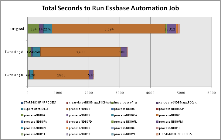
First of all, take a look at the below graph:

Total Seconds to Run Essbase Automation Job

Total Seconds to Run Essbase Automation Job

What you’re looking at is a graph that has been created in Excel, based on data in a text file that was generated as a result of a profiling process.  The steps are as granular as we want them to be.  In other words, if we simply want to clump together a bunch of jobs that all run really fast, then we can do that.  Similarly, if we want to break down a single job that seems to take a relatively long amount of time, we can do that too.  Each segment in the starcked bar chart is based on the number of seconds that the particular step took.  We can see that in the original (pre-optimization) scenario, the orangey-brown step takes up a pretty considerable amount of the overall processing time.  After some tweaking, we were able to dramatically slash the amount of time that it took to run the whole job.  And, in the third bar, after yet more tweaking, we were able to slash the overall processing time quite a bit again.

The important thing here is that we are now starting to build an understanding of exactly where we are spending our time — and we can therefore prioritize where we want to attempt to reduce that time.  My next post will detail a sample mechanism for getting this kind of raw data into a file, and the next few posts after those will start to dig in to where and how time was shaved off due to better outline, system, and other settings and changes.  Happy profiling!