jason w. jones

software from the trenches

Multiple Applications in Dodeca

I want to talk about one of the more interesting aspects of Dodeca and its extensibility: applications. In some of my past posts, I’ve alluded to this notion of applications (and also something called a tenant) in Dodeca but haven’t really had a chance to dive into much detail. I’ll get into the notion of tenants some other day, so today’s focus is on what an application is.

In our world (the EPM world, that is), the term application has a lot of meanings. In Essbase-land, it’s a container for cubes or plan types. In the world of software, it usually means a single program. In the world of Dodeca, an application defines the views, behavior, look, and other properties that a user will see when they launch Dodeca.

More specifically, consider that when you login to Dodeca, you are actually logging in to a specific Dodeca application (whether you realized it or not). Typically on the left side of the Dodeca window is the list of views that you have access to. This list of views is called the view selector. Now, the view selector itself has several options that determine which views are shown to a given user, but for now just let’s just think of the whole thing (irrespective of content) as the view selector.

Additionally, when logging in to Dodeca, it’s quite common to use your enterprise credentials (your username and password) that give you access to a given Essbase server and other things around the company. Interestingly enough, the authentication strategy in Dodeca can be configured on a per-application basis. This means that you might want to use a particular cube to authenticate users in one app, but use a different cube, or LDAP or Active Directory, or something else entirely, to control authentication in another application.

If this feels like an amazing amount of configurability to wield, that’s because it is. Many (most?) software programs that allow for enterprise login capabilities (that is, logging in against an LDAP or similar server) tend to have that configuration buried in a configuration file somewhere, and they only support a global authentication provider configuration.

Now that we know a little about what an application is, let’s take a look at the process of creating an new application. As with most objects in Dodeca, Applications have their own menu item under Admin, which brings up a list of apps that can be edited. From there, it’s a simple matter of just selecting New and typing in some details:
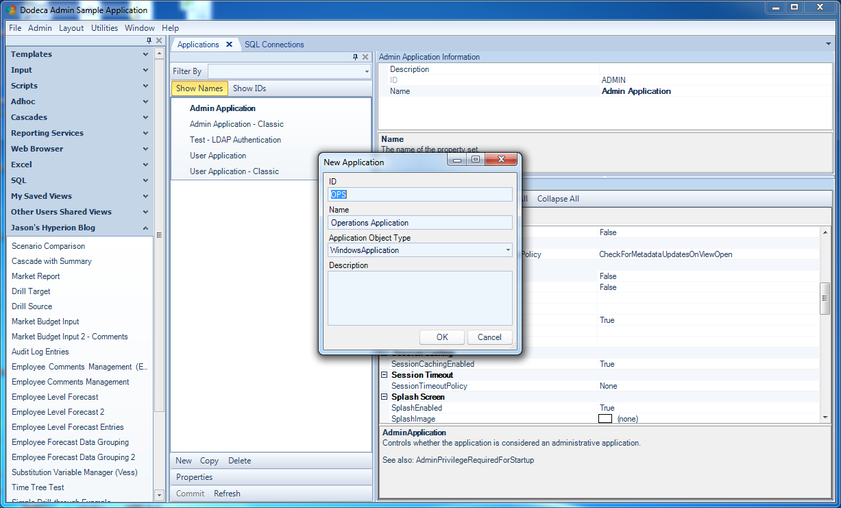
Creating a new application in Dodeca

Creating a new application in Dodeca

Let’s give this application an ID of “OPS” – we’ll assume for this example that Dodeca has heretofore been used just in the Finance group, but that the folks in Operations saw how productive and happy the Finance people were and they want to get in on some of that sweet 12-sided action. Also, it’s customary for the application ID to be all capitals and not contain any spaces, as it will be referenced in URLs and shortcuts. We can give it a nicer name, however, which in this case will be “Operations Application”.

Next, we need to configure some essential properties for the application. There’s a lot we can configure, but for now we’ll stick to the basics. First up, let’s change the caption for the app (the text shown for the titlebar of the program window):
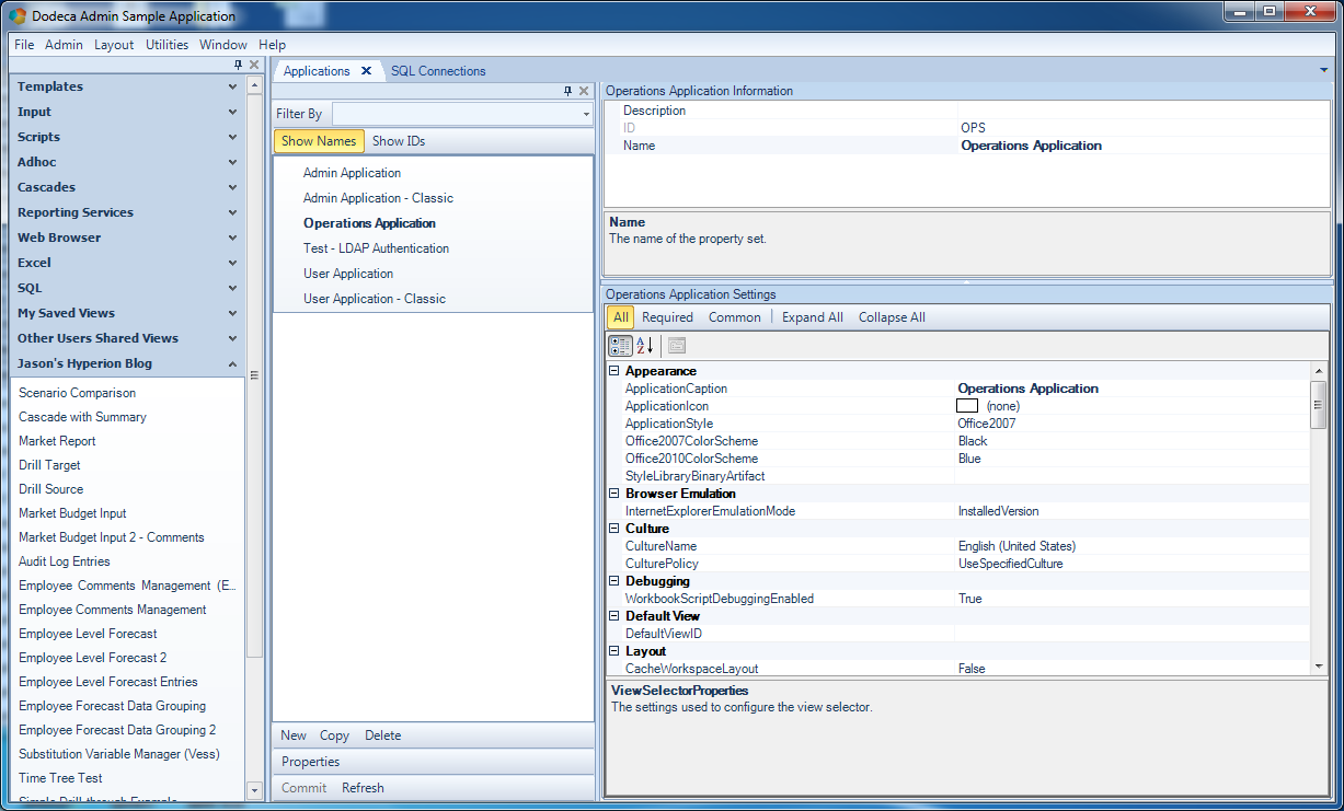
Configuring properties for the new application

Configuring properties for the new application

Remember, bold properties are the ones that we’ve changed from the default, so in this screenshot I’ve only changed the caption. Next, let’s set the authentication properties:
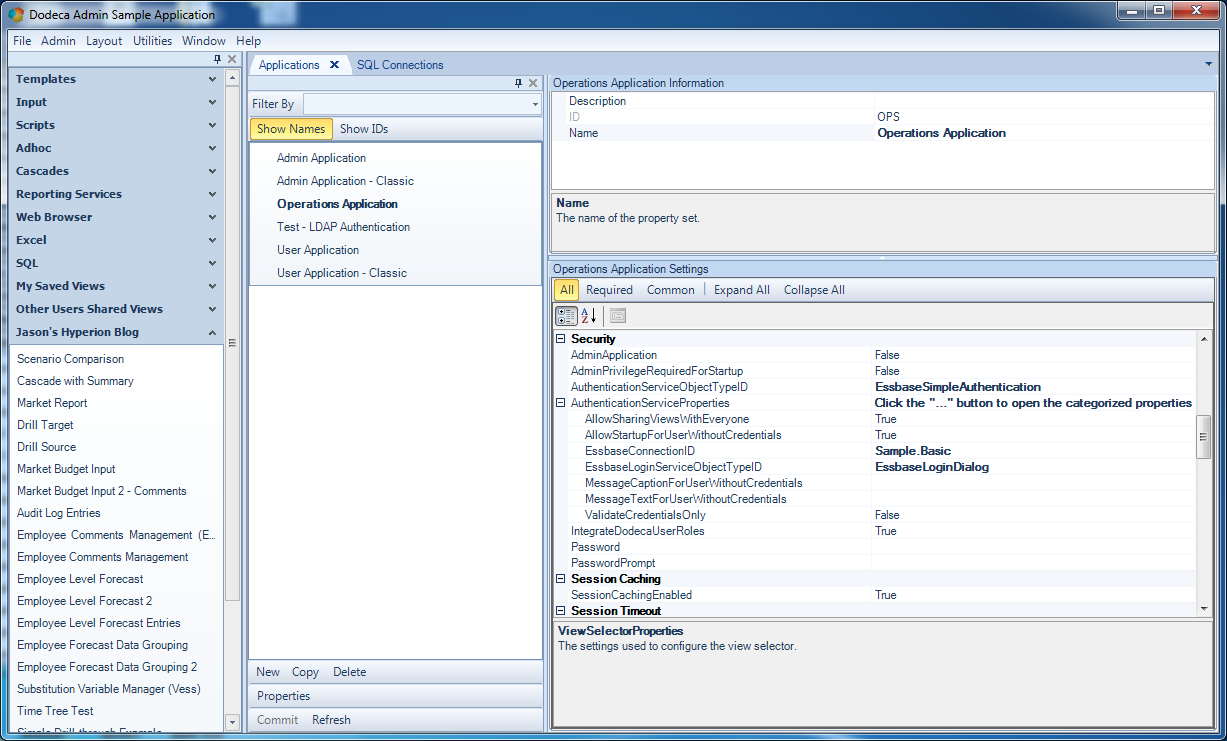
Configuring the authentication strategy for the app

Configuring the authentication strategy for the app

There are several choices here. One of the more common and useful is the EssbaseSimpleAuthentication service. This essentially means that a given cube (one of the defined Dodeca Essbase connections) will serve as the object which is logged into in order to validate a user. The EssbaseConnectionID setting is simply a dropdown where we can quickly select an existing connection.
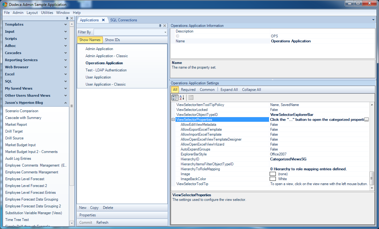
Setting the view selector and hierarchy for the application

Setting the view selector and hierarchy for the application

Next, we configure a view selector. For this application we’ll just go with a ViewSelectorExplorerBar, then choose a HierarchyID (again as a refresher, hierarchies are also defined in Dodeca as with other objects). That’s actually all we need for now. Since I’m just using an existing hierarchy for demonstration purposes, I expect the contents of the hierarchy in the new application to be the same contents as what I see in this existing application used in the screenshots.

After committing the changes, the new application is ready to be used. In my environment, I can launch it with the following launching the URL http://dodeca:8080/dodeca/smartclient/AppliedOLAP.Dodeca.SmartClient.application?t=SAMPLE&a=OPS

Note that I just took an existing URL and changed the last parameter (...a=OPS) so that it points to the OPS application. Upon launching the URL, my new application comes up and I can run a view in there as I normally would:
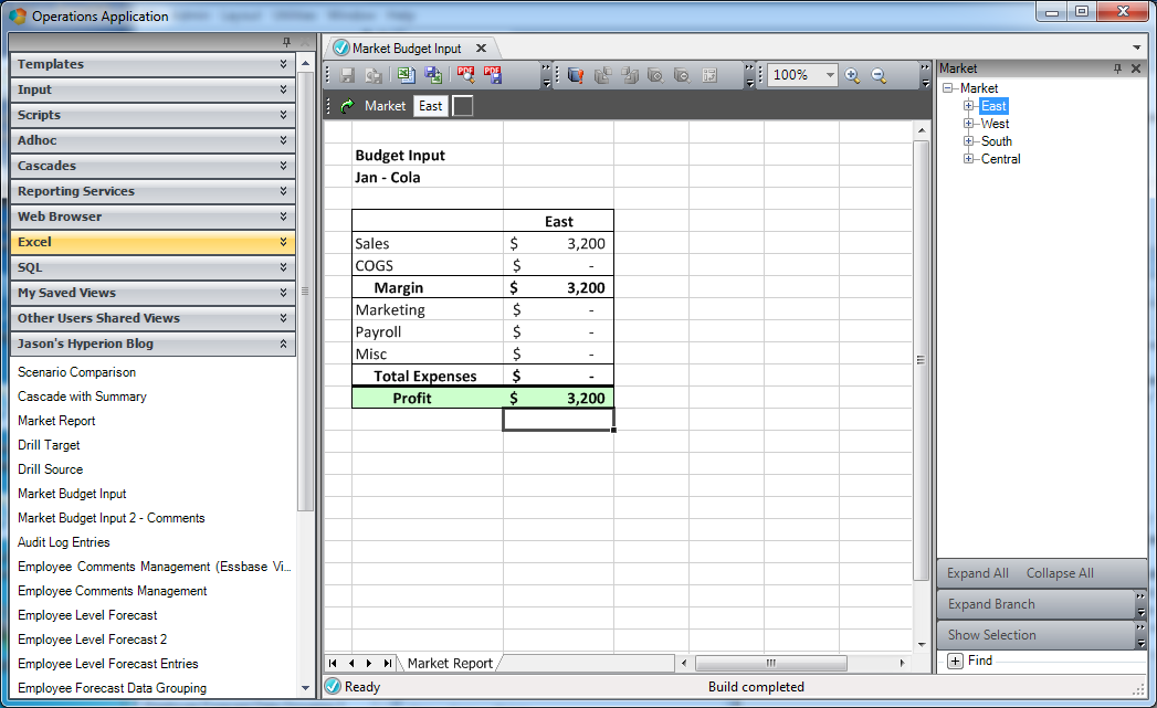
The newly created application has been launched and a report built

The newly created application has been launched and a report built

You may notice that the look of this application is different than the one we were just in. This is just configured on the application properties. While I didn’t change the look of the new application from the defaults, as it turns out, the app we’ve been working in to this point does have a custom style, so that’s the reason for the difference.

Dodeca Applications Summary

Dodeca has an even greater form of partitioning functionality (called tenants) that I’ll cover in the near future, but I hope this gave you an interesting since of some of the power inherent in the Dodeca application model. I think it’s incredible that we’re able to rapidly spin up a completely distinct Dodeca application by just configuring a few properties. One thing to keep in mind is that this didn’t require setting up a new Dodeca server, a new Dodeca repository, installing software or anything. It’s just modularity that’s inherent to the design of the software. Applications can be used to provide specialized behavior for different groups, sub-groups, types of users, divisions, or whatever else makes sense.

Greet your Dodeca users with a custom landing page

Today’s Dodeca post will be on the lighter side, but is nonetheless a pretty useful feature. One of the interesting aspects of Dodeca is its support for multiple tenants and applications. This means that within just a single Dodeca repository (created when the Dodeca service is installed), we can have multiple distinct applications. This allows for creating different applications for different groups of users. It’s really quite powerful and something I will explore more in the coming weeks.

That said, since we can organize Dodeca into multiple distinct applications, that also means we can configure the properties of each application however we want. And one of those settings we can configure is the default view. The default view is a normal Dodeca view that is opened automatically when the application is launched.

Imagine that you want to have different applications for different groups. For instance, you might want an application for Finance, an application for Operations, and something for the Marketing department. As with just about all other objects in Dodeca, Applications are managed with their own editor, just as one would edit a View or Selector. Here’s a look at the four applications I have in my demo instance right now:

Setting properties for the Dodeca application itself

Setting properties for the Dodeca application itself

You might notice that on a per-application basis, I can control the style/theme of the app, and some other things. As I mentioned, one of those things (and the topic of this post) is DefaultViewID. With this setting, we can tell that Application that when it’s launched, it should run a particular view and open it up. This can be used as a sort of start or landing page for your users. And remember, this is controlled per-app if we want: meaning that we can have different default views for different groups of users, as it makes sense.
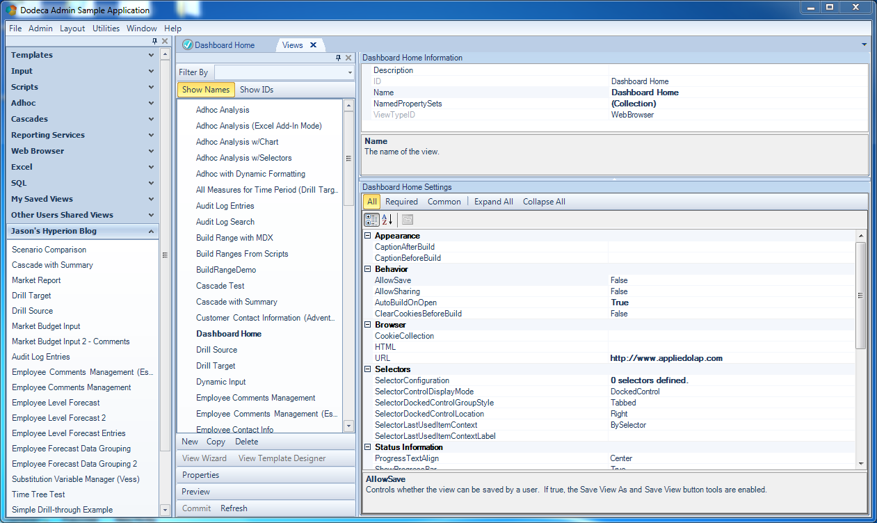
Most of the views that I have blogged about in the past have been one of two types of views: either an Essbase Excel view, or a SQL Excel View. But there are actually a handful of other view types, one of which is a Web Browser view. This view type is pretty straightforward. Whereas Essbase views concern themselves with Essbase data and retrieves, the web view is mostly just concerned with showing some HTML or fetching a particular URL.

You may notice in the above screenshot that I have set the default view for this app to Dashboard Home. This is a new web view that I will setup in the next couple of steps.

The following screenshot shows the properties for a simple web view that opens up the Applied OLAP home page. If you look at the non-default properties I have set, I turned on AutoBuildOnOpen (so the web page is fetched when the view is opened) and specified a URL:

Dodeca configuration for a WebBrowser view

Lastly, I have the WindowsViewUIObjectTypeID set to WebBrowser, which is the last property I need to set in order for this to work:

Part 2 of the view properties available for a web view

Part 2 of the view properties available for a web view

Now to tie it all together. Given that I have created a new web view and set it as the default view for the application, here’s what I am greeted with now if I close and open this application:

Dodeca configuration for a WebBrowser view

Dodeca client with a Web View displayed

Dodeca client with a Web View displayed

Hopefully the use case for this isn’t too hard to imagine. The most common usage of this type of dashboard/default view that I see is to point it to a group-specific intranet page that has information about the status of Essbase, the current financial period, and links to metadata-related activities (like requesting a new member to be added to an outline or something).

Playing with the Thriller MDX/JDBC Driver in Drillbridge

Last week I talked about a new side project, which is a JDBC driver called Thriller for executing MDX queries against Essbase and mapping the results back into a normal relational database. And at the time, I said that this driver had some really interesting use cases, such as in Dodeca, Drillbridge, ODI, and other tools that work with JDBC drivers.
Speaking of Drillbridge – in the very near future I will be sharing Drillbridge’s official future direction, which I think is really exciting, but more on that later. In the meantime, let’s drop this baby into Drillbridge and see what happens!

The following walkthrough of using Thriller with Drillbridge will show off some features that are only available in the licensed version of Drillbridge, although this should in theory work with Drillbridge Community Edition (the free edition of Drillbridge), assuming you have the Thriller driver JAR file.
First of all, with the Thriller driver file having been placed in the /lib under the Drillbridge installation folder, we can restart Drillbridge and navigate to the Connections screen:

Overview of connections in Drillbridge

Overview of connections in Drillbridge

Recall that in Drillbridge, Connections represent the list of potential relational databases/schemas that we might want to use to execute a query against. Since the Thriller driver makes a relational database facade for us, we are going to treat it just like any other relational database connection, such as Microsoft SQL Server Oracle, MySQL, DB2, or whatever. You may notice in the above screenshot that there is already an entry for Sample/Basic using the Thriller driver. I already added it, but let’s go take a look at the connection configuration itself:

Editing a new Drillbridge connection with the Thriller MDX/JDBC driver

Editing a new Drillbridge connection with the Thriller MDX/JDBC driver

There’s nothing too special here – a name, credentials, and probably most importantly, a particular JDBC URL that is specific to Thriller. The general syntax for the Thriller JDBC URL is jdbc:essbase:thriller://server/Application.Database. Note that at the moment, Thriller assumes an “embedded” Essbase connection strategy (as opposed to going through APS).

As with a normal relational database connection, we should verify it to ensure connectivity and proper credentials:

Testing the Thriller MDX/JDBC connection

Testing the Thriller MDX/JDBC connection

With the connection now created, we can move on to creating the Drillbridge report, which will reference that connection. Let’s create a new report and edit the essential fields:

Creating a Drillbridge Report with a Thriller MDX query

Creating a Drillbridge Report with a Thriller MDX query

You can’t see the entire interface, but the essentials are shown: I have set the connection for this report to use the new Thriller connection to Sample/Basic, and I have dropped in a specifically crafted Thriller query. The comments with the column names/types are part of the Thriller mechanism for mapping MDX results to a flat result set. If you want crash course in how it works, please head over to the introductory blog post where I showed how to make George Spofford cry make it work.

So, we have our driver in place, a connection setup, and a new report created that specifies that connection and a specially crafted MDX query. That’s actually all we need for now to see this thing in action. Let’s go over to the Test tab:

Testing the Drillbridge report

Testing the Drillbridge report

There are no tokens in the query (yet), so there is nothing to specify, so we can bit the Build It! button, cross our fingers, and see what happens. And wouldn’t you know, data comes back, per our column mapping specification:

Thriller/Drillbridge query output

Thriller/Drillbridge query output

Nice.

Let’s go for extra credit by parameterizing one of the members in the query and use the new Drillbridge token editor interface. Back over in the query, let’s take out Cola and drop in a “short token”:

Adding a "short token" to the Thriller MDX/JDBC query

Adding a “short token” to the Thriller MDX/JDBC query

If you look carefully, you’ll notice that Cola from the original query is replaced with {{#Product}}. This is known as a “short” token in Drillbridge. This is mostly useful so you can quickly drop it in and then use the token editor to customize the token. With the token in place, let’s navigate over to the Tokens menu:

Navigating to the Token editing interface

Navigating to the Token editing interface

This will show us all of the recognized tokens in our query:

The Edit Tokens interface displays the recognized tokens in the query

The Edit Tokens interface displays the recognized tokens in the query

There’s just Product so we can click on it and bring up the options for this specific token:

Editing options for the Product token

Editing options for the Product token

We don’t really need to change anything here, but let’s drop in a Sample Value so that it will pre-fill the box when we go to test the report. Updating the token results in the corresponding query being updated:

Query updated with token options

Query updated with token options

Notice that the short token got replaced with a full token (JSON syntax). We can now go test the report again and see that we now have a token we can customize:

Testing the report again, now with a Product token

Testing the report again, now with a Product token

Although the screenshot shows Cola (since that came up by default, for testing purposes I actually put in the value of another product, Sasparilla). Press build, and then:

The built report (using a different product)

The built report (using a different product)

The eagle-eyed amongst you might notice that this data is different than before (as it should be, since it’s a different product). Just for fun and to finish things out, let’s click on the Excel button to download as an Excel (.xlsx) file, as we would with any other result set coming from a JDBC/relational database:

Drillbridge report downloaded to Excel

Drillbridge report downloaded to Excel

As with the normal Excel output generation, Drillbridge has inspected the data types of the columns (VARCHAR/String, DECIMAL, INTEGER, etc.) to try and find the best matching Excel column type. So, nicely enough, the values in columns B through D, corresponding to Jan, Feb, and March, are true Excel numeric values (as opposed to labels).

The Drillbridge/Thriller Use Case

Now, you might be thinking, wait, why would I need to drill in to Essbase data… from other Essbase data? In other words, if you’re navigating the cube using Smart View, why on earth would you need to drill in to data that’s already in the cube? There are some edge use cases where I think this could be useful, but actually what might be much more useful is that you could use this to drill into data that’s in another cube. So maybe you have some cubes with common but different dimensionality. There’s nothing stopping you from dropping in a drill-through definition with Drillbridge that let’s you drill from the cube, over to Drillbridge, where it then runs this query and displays the results. You could, of course, use the Drillable Columns feature in Drillbridge to drill from/between different Drillbridge reports based on the POV of a row in the column result set.

Interesting… and Useful

I have repeatedly referred to this driver as well as other flights of fancy (Vess) as being “interesting”. That’s kind of my way of saying, “Yeah, it works, technically… but is it the best solution?” I think this use case with Thriller tips the scales from just Interesting over to actually useful, as I can see some pretty useful opportunities where this could be dropped in and get quick win.

I’m still working out a few kinks with the driver, but to those of you that emailed to get an early copy to play with, I say thank you – and please hang on for a bit as I clean a few things up and make this more generally useable.

Running MDX queries through a JDBC driver (for fun?)

So there I am, sitting in front of the Alaska Airlines gate at Boston Logan airport, waiting for my flight home to Seattle. It’s not a particularly glamorous terminal – the divorce from Delta hasn’t been too kind to Alaska at BOS; Delta seems to have kept the house and kids while Alaska microwaves Lean Cuisine on a futon in its bachelor pad…

As I’m pondering why there are white rocking chairs in the terminal, my phone rings with a familiar name: Mr. Brian Marshall. We catch up and exchange pleasantries before pivoting over to more important matters (all things EPM of course!).

Brian: “So… Vess.”

Jason: “Oh boy…”

So we get to talking about accessing Essbase data through a Java database driver, á la Vess. And we get to talking about running MDX queries and dumping the output – á la Camshaft.

And as the talk goes on I end up saying something stupid like this: “You know what might work? Jjust pass an MDX query through the driver over to Essbase and map the output to a fake table… It’d be like an unholy combination of Vess and Camshaft. You could probably knock it out in a day or two.”

And at that moment I knew I wouldn’t be able to resist opening my laptop for the five plus hour flight home.

Vess + Camshaft = ?

So, what if we write a custom JDBC driver that takes a normal MDX query and some hints about how to convert the output to a regular table, run it against an Essbase cube using the Essbase Java API, and then process the results so they look like a normal table? Could we drop that into any old JDBC tool or software (Dodeca, Data Visualization Desktop, Java programs) and have it work?

Well, yeah. Now, that doesn’t mean that it’s a good idea. But it most certainly works. Here’s an example:


/**
* Pull first quarter measures for Cola for total market
*
* -- column.1.name = MEASURE
* -- column.1.type = VARCHAR
* -- column.2.name = JAN
* -- column.2.type = DECIMAL
* -- column.3.name = FEB
* -- column.3.type = DECIMAL
* -- column.4.name = APR
* -- column.4.type = DECIMAL
*
*/

SELECT CROSSJOIN({[Jan], [Feb], [Apr]}, {[Cola]}) ON COLUMNS,
{[Measures].Levels(0).members} ON ROWS FROM [Sample].[Basic]

As you can see, I have a normal MDX comment block and an MDX query. Inside the comment block is where we can “stash” some parameters or hints to the query parser so that it knows how to map the output. To some extent the driver could try and infer what the column names, types, and other attributes should be, but at least for prototyping purposes, I think explicitly defining them is the way to go.

Upon executing the query against our favorite database in the world (Sample/Basic!), we get the following results (printed to text on the console in this case):


+--------------------+--------------------+--------------------+--------------------+
|MEASURE             |JAN                 |FEB                 |APR                 |
+--------------------+--------------------+--------------------+--------------------+
|Sales               |4860.0              |4821.0              |5048.0              |
|COGS                |1888.0              |1886.0              |1949.0              |
|Marketing           |667.0               |673.0               |699.0               |
|Payroll             |586.0               |586.0               |596.0               |
|Misc                |9.0                 |10.0                |11.0                |
|Opening Inventory   |14587.0             |14039.0             |13660.0             |
|Additions           |4312.0              |4348.0              |5560.0              |
|Ending Inventory    |14039.0             |13566.0             |14172.0             |
|Margin %            |61.152263           |60.879486           |61.39065            |
|Profit %            |35.185185           |34.557146           |35.519017           |
|Profit per Ounce    |142.5               |138.833333          |149.416667          |
+--------------------+--------------------+--------------------+--------------------+

Of course, being MDX we aren’t limited to just data from the cube itself, we can even ask for dimension properties and information. For example, consider the following MDX query that runs against Sample/Basic and asks for the member name, alias, and level of members in the Product dimension:


/**
* Pull alias and level informatin for products
*
* -- column.1.name = MEMBER_NAME
* -- column.1.type = VARCHAR
* -- column.2.name = ALIAS
* -- column.2.type = VARCHAR
* -- column.3.name = LEVEL
* -- column.3.type = INTEGER
*
*/

SELECT {} ON AXIS(0),
Product.Members DIMENSION PROPERTIES
PROPERTY_EXPR (Product, MEMBER_ALIAS, CurrentAxisMember(), "Alias"),
PROPERTY_EXPR (Product, LEVEL_NUMBER, CurrentAxisMember(), "Level")
ON ROWS
FROM Sample.Basic

After executing, we get the following data:


+--------------------+--------------------+--------------------+
|MEMBER_NAME         |ALIAS               |LEVEL               |
+--------------------+--------------------+--------------------+
|Product             |                    |2                   |
|100                 |Colas               |1                   |
|100-10              |Cola                |0                   |
|100-20              |Diet Cola           |0                   |
|100-30              |Caffeine Free Cola  |0                   |
|200                 |Root Beer           |1                   |
|200-10              |Old Fashioned       |0                   |
|200-20              |Diet Root Beer      |0                   |
|200-30              |Sasparilla          |0                   |
|200-40              |Birch Beer          |0                   |
|300                 |Cream Soda          |1                   |
|300-10              |Dark Cream          |0                   |
|300-20              |Vanilla Cream       |0                   |
|300-30              |Diet Cream          |0                   |
|400                 |Fruit Soda          |1                   |
|400-10              |Grape               |0                   |
|400-20              |Orange              |0                   |
|400-30              |Strawberry          |0                   |
|Diet                |Diet Drinks         |1                   |
|100-20              |Diet Cola           |0                   |
|200-20              |Diet Root Beer      |0                   |
|300-30              |Diet Cream          |0                   |
+--------------------+--------------------+--------------------+

From a SQL/JDBC perspective, the columns all have the types that we specified in the “hint” section: the MEMBER_NAME and ALIAS fields are VARCHAR columns, and the level is a plain INTEGER.

Use Cases

There are a number of places I think this driver could be applied usefully:

  • Extracting metadata with a query tool/engine
  • Using MDX data in a Dodeca SQL Passthrough DataSet
  • Drilling to MDX query data in a tool that understands JDBC (Drillbridge et al)

Extracting Data/Metadata

Conceptually, this use case is approximately the same as just using MDX to extract data using MaxL or with Camshaft, but you could potentially save yourself the step of having to then load that text file into a database. This could potentially come in handy for some use cases where you don’t want to deal with the file system.

Using in a Dodeca SQL Passthrough DataSet

Dodeca already supports MDX in various ways and due to its inherent power and flexibility, MDX is being creatively used in a rapidly growing number of use cases. This is provided by way of various BuildRangeFromScript Workbook Script methods. That said, as is true for other tools out in the world, JDBC data/connectivity is already a first-class citizen in Dodeca, so this driver opens up the interesting possibility where we could treat MDX data/metadata as just any other normal table/view.

This approach wouldn’t necessarily be better, but it could open up some very, very interesting possibilities where the MDX data is loaded up in a DataTable range on a view and, for example, Dodeca’s declarative dynamic grouping/sorting/filtering is applied on the fly. I’ll likely show an example of this in the near future.

Drilling to MDX Data (Drillbridge!)

In addition to the classic “JDBC Drillthrough Report” that is the workhorse of Drillbridge, the enhanced version of Drillbridge ships with two other report types (in addition to supporting custom plugins): link-based reports and MDX query reports. In Drillbridge, the MDX query report is used to generate and execute an MDX query instead of a normal SQL query, then the grid-based results are displayed to the user.

Given that all versions of Drillbridge support third-party JDBC drivers, this driver could be particularly interesting to drop in to Drillbridge, then run a normal MDX query and display the results in a completely columnar format. I’ll also probably show an example of this in the near future as I think it could be really cool.

Availability & Next Steps

I’ll use the same word to describe this software as I did for Vess: It’s interesting. This driver is a bit more “unholy” than Vess in some ways since it’s trying to pretend one thing (OLAP data) is another thing (OLTP data). Just for the record, I fully, fully, fully realize that among other things, MDX was invented because OLAP databases are altogether a different animal than relational databases. But it’s quite likely that JDBC is much more common than MDX (or rather, there are more tools that inherently work with JDBC than its equivalent for OLAP databases).

Just email me if you’d like to take the driver (Java JAR file for a spin). As with Vess, it’s incredibly experimental but it works surprisingly well. You’re free to play around with the JAR file and hopefully provide feedback on any kinks you run into (oh, and blog about it, that’d be cool too).

New Indenting Options in Next Generation Outline Extractor writer

Besides talking about and working on all things Dodeca Spreadsheet Management System, Dodeca Excel Add-In, and Drillbridge, one of the other things I am helping with these days at Applied OLAP is continuing work on the Next Generation Outline Extractor.

Most readers of this blog are probably familiar with the outline extractor. Almost everyone I know in the EPM world uses it or has used it in the past. It is an incredibly popular tool and I am very proud to contribute my efforts to making it even better.

As a quick aside, I want to point out that having been with Applied OLAP for some time now, I can say that the Outline Extractor is truly a community tool: it is absolutely free, downloaded tens of thousands of times, used by countless developers and admins, and perhaps most amazing of all, Applied OLAP supports the tool. Emails come in all the time with with questions on how to download and use this tool, and without fail, the exceptional Applied OLAP support team quickly jumps in to get the user up and running. So, I must say that it’s amazing to see and take part in an organization that supports its community so whole heartedly.

That all said, some of those emails, phone calls, and general interacting with people at conferences at Kscope are related to one-off feature requests, which is more my department (yes!). If there is something you’d like to see in the outline extractor, please don’t hesitate to let us know. Better yet, send a tweet to @AppliedOLAP and/or @jwj and get the discussion going.

In the meantime, I’d like to point out a small improvement to the outline extractor that will be available to download soon. It’s a new indenting option for the Documentation Text Writer plugin that allows you to indent the output by generation, as well as specify the text that is used to indent.

I’ll show you how it works. The screenshots might seem a bit foreign since I’ll be running the extractor on my Mac (that’s right, the extractor runs on macOS!).

First, for the sake of the demo, let’s connect to a an EPM server, choose Sample/Basic, and just pick a single dimension to output:

Choosing dimensions to output in the Next Generation Outline Extractor

Choosing dimensions to output in the Next Generation Outline Extractor

For the output, I’m only going to select the Documentation Text Writer (which is the particular output writer that has the new option):

Choosing the output plugin(s) in the Outline Extractor

Choosing the output plugin(s) in the Outline Extractor

You might also note that the default output directory (shown above) is to a /output subfolder. This is also a small new feature. By default, the Outline Extractor will now try and put output in a local /output folder, to keep things a little cleaner.

Now let’s turn on the new option:

New generation indent and indent text settings in Documentation Text Writer

New generation indent and indent text settings in Documentation Text Writer

You might notice that I turned all other options off (I deselected their checkboxes). This is for a couple of reasons, one, I want to just show off the new output option, but I also want to show what’s possible with the outline extractor’s myriad options for output. A lot of people use this tool to get exactly the output they need, whether it be for automation, some validation process, inputting data into another system, or something else. The user requesting this new indenting feature wanted to be able to get a “clean” hierarchy from a cube, and this is how you can do it.

Notice that the indentation text is \t. This corresponds to the tab character. So however deep a member is in the hierarchy, it’ll be indented with that character the number of levels deep that it is. After running this extraction, let’s take a look at the output:

Indent generations feature applied to Sample/Basic Year dimension output

Indent generations feature applied to Sample/Basic Year dimension output

There you have it: a nice, simple, “clean” output of the dimension. It’s a small improvement, but there are a surprising number of extractor use cases that revolve around outputting dimension information so that a user/admin can simply “eyeball” it for any obvious issues, and indenting significantly helps with that.

So, just a small improvement for now, but there’s more in the pipeline. As I said, please don’t hesitate to let us know about your ideas for improvements. We can’t promise to make them right away (priorities!) but for the absolute least part, they’ll be taking into consideration. At the moment, the public download of the Next Generation Outline Extractor does not include this improvement – it’ll be available in the coming days. I’ll post about it when it’s publicly available!


Dodeca Techniques – Auto Load Windows User Name During Relational Input

Today I want to look at a practical example in Dodeca that came up while I was at a Dodeca training workshop for a client the other week. We know that Dodeca can update data in a relational database using its robust SQL Passthrough DataSet functionality. And we know that it can automatically use values from the selectors to update columns as needed (for example, if the user has selected a Scenario of Actual, we could use a token such as [T.Scenario] in the SQL query).

Now let’s say that we have a table with data, such as headcount forecast data, and for whatever reason (auditing), we want to record the username of the user that is inputting the data. To achieve this, we can use a single Workbook Script method and a function to dynamically insert the Windows username of the current user into the view, and then use that token just as we would use any other token. In this case, we’ll use that token in the INSERT/UPDATE statements on the SQL Passthrough DataSet. Note that none of this configuration has anything to do with security, per se, it’s purely to have a column in the table to make it easy to see who updated/inserted a given piece of data.

In the following steps, I am going to create the SQL Passthrough DataSet (for defining how Dodeca should select, insert, and update data in a simple relational table), lay out the SQL Excel View template (with a named range to be filled with data), set a few options, create a simple workbook script, and then test things out. Here goes:

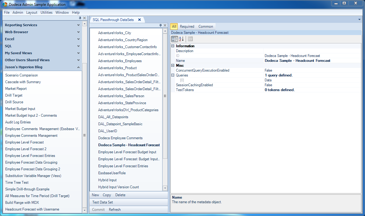
First things first, we need to make the SQL Passthrough DataSet. The following screenshot shows the overview for this object, mostly shown just for completeness (as the main configuration happens inside of the Query definition). But here you can see that this SQLPTDS has one query defined:

SQL Passthrough DataSet properties

SQL Passthrough DataSet properties

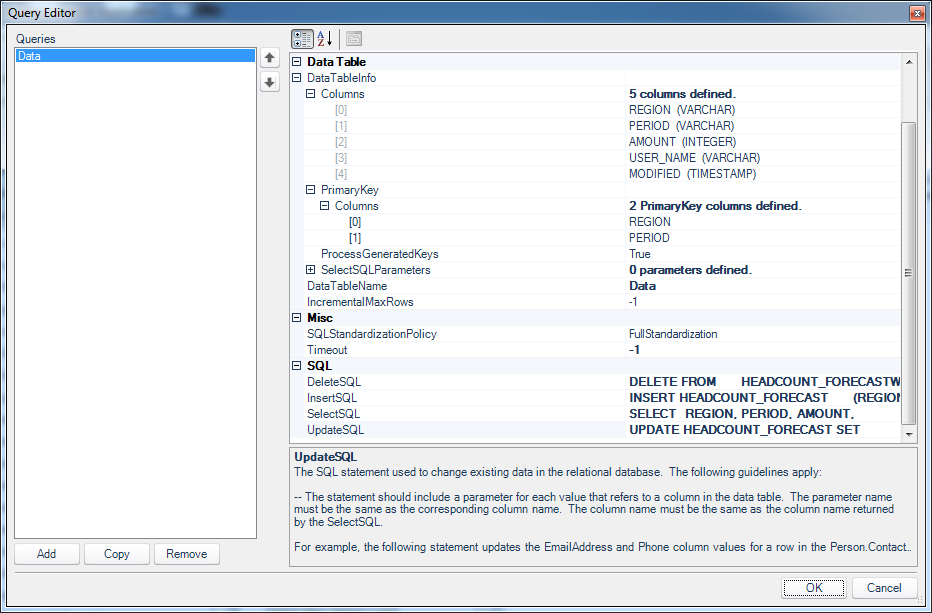
Now for the query definition:

Editing the query for updating, adding, selecting, and deleting "headcount forecast" entries

Editing the query for updating, adding, selecting, and deleting “headcount forecast” entries

You can see that I’ve laid out the columns for this simple table (this isn’t always strictly necessary but it doesn’t hurt), the compound primary key (REGION + PERIOD), a name to link it to the view (DataTableName = Data), and the four SQL templates for deleting, inserting, selecting, and updating.

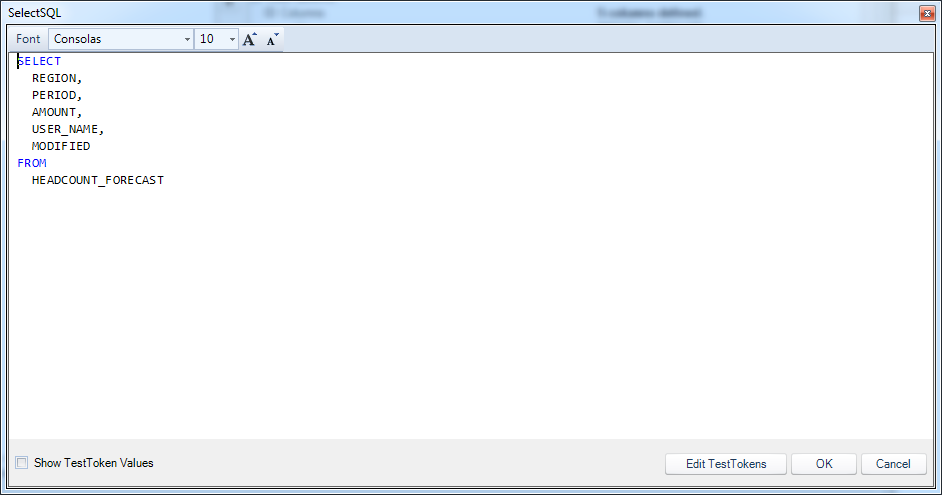
Here is the code for selecting records from the table:

The SELECT query for the headcount forecast data

The SELECT query for the headcount forecast data

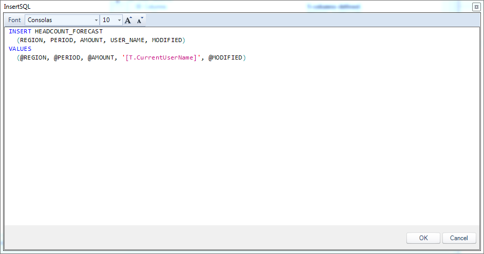
And for inserting new ones:

The query for inserting a new headcount forecast entry

The query for inserting a new headcount forecast entry

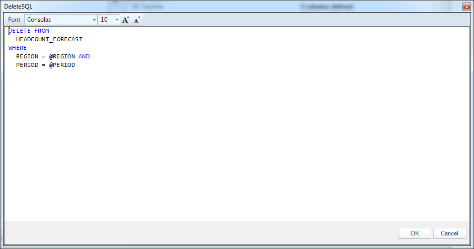
For deleting ones:

Deleting a headcount forecast entry

Deleting a headcount forecast entry

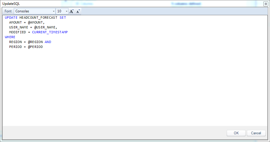
And for updating them:

The code for updating a headcount forecast entry

The code for updating a headcount forecast entry

Of these statements, the INSERT is the most interesting. You can see that we are using the [T.CurrentUserName] token. I’ve shown various examples before that insert with tokens, but the difference this time is that this token isn’t one that comes from a selector on the view (indeed, this view doesn’t have any selectors). This token will be created when the view is opening using some custom Workbook Script that we’ll setup in just a moment. As another nicety in terms of populating this audit type data into the table, we use the CURRENT_TIMESTAMP function to fill the MODIFIED column. Note that the CURRENT_TIMESTAMP function is native to MySQL databases. For Oracle and Microsoft SQL Server, you’d use a different function.

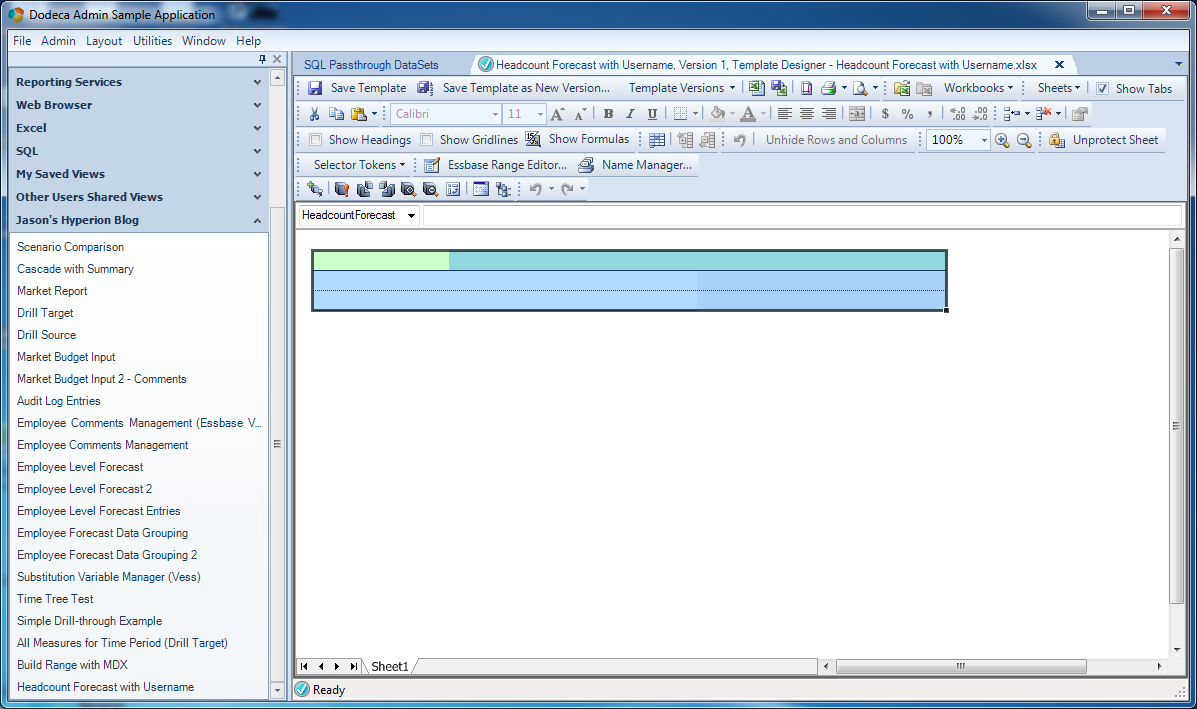
With the SQL Passthrough DataSet configured, we can now go create the view template:

Excel template configuration for the headcount forecast editing area

Excel template configuration for the headcount forecast editing area

The main thing here is the named range that will be populated with data from the SQL table. In this case, it’s three rows tall. This is the size you make a named range when you are going to retrieve the SQL data along with the headers (column labels). If you don’t bring back the headers, then you’d want to make this just two rows tall. You can see that I have named the range (HeadcountForecast). As additional superficial formatting, I have turned off row and column headers on the spreadsheet and turned off gridlines. It may be hard to tell but if you look closely you can see that I made the last two columns of the range light grey. These columns correspond to the user name and the modified time of the row. I don’t allow the user to edit these so I have changed their color.

Again, you can’t really see it but one other thing I did was turn off cell protection for the first three rows of the named range (this is configured using a checkbox on the properties for a cell/range), and I turned on “Protect Sheet”. The effect of this is that the user will only be able to edit cells I designate. This is one of the “quieter” but amazing features in Dodeca: we can retrieve SQL and Essbase data into a sheet however we want, and lock any cells we want. In addition to the cell background color being grey and offering a visual cue that data is not editable there, we can just lock the cells entirely to prevent changes, and prevent the user from thinking that they should be able to or want to change the data.

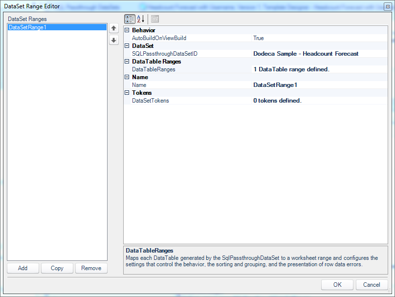
With the template all setup, we can now turn our attention to the view configuration. The view configuration is pretty standard, so I’ll jump right into the DataSet Range editor (part of the SQLPassthrough DataSet configuration on the view):

dodeca-auto-load-user-name-08-view-datasetrange-editor

The DataSet Range editor

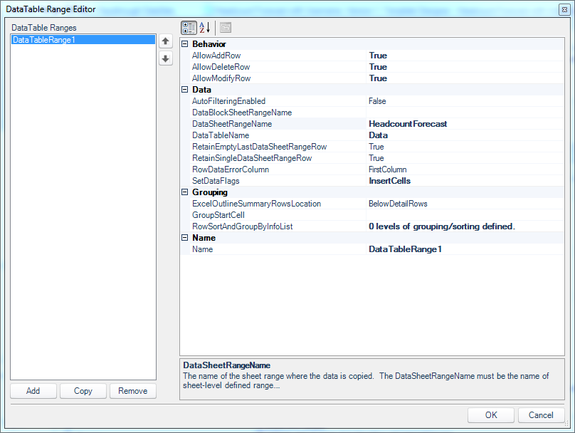
Here you see that I just have the one DataTable defined for the DataSet. Also notice that I have chosen the proper SQLPassthroughDataSetID from earlier. Now inside the DataTable Range Editor:

The DataTableRange Editor within the DataSet Range editor.

The DataTableRange Editor within the DataSet Range editor.

As with examples I’ve shown before, I have turned on the ability to add, delete, and modify rows, specified the corresponding named range on the Excel template, set the proper DataTableName from earlier, and configured SetDataFlags to InsertCells (so that when the view is built, the data from the SQL table will effectively be “inserted” into the view, thus extending our formatting and preserving cell references across the sheet).

Let’s take a quick look at the view properties for this view:

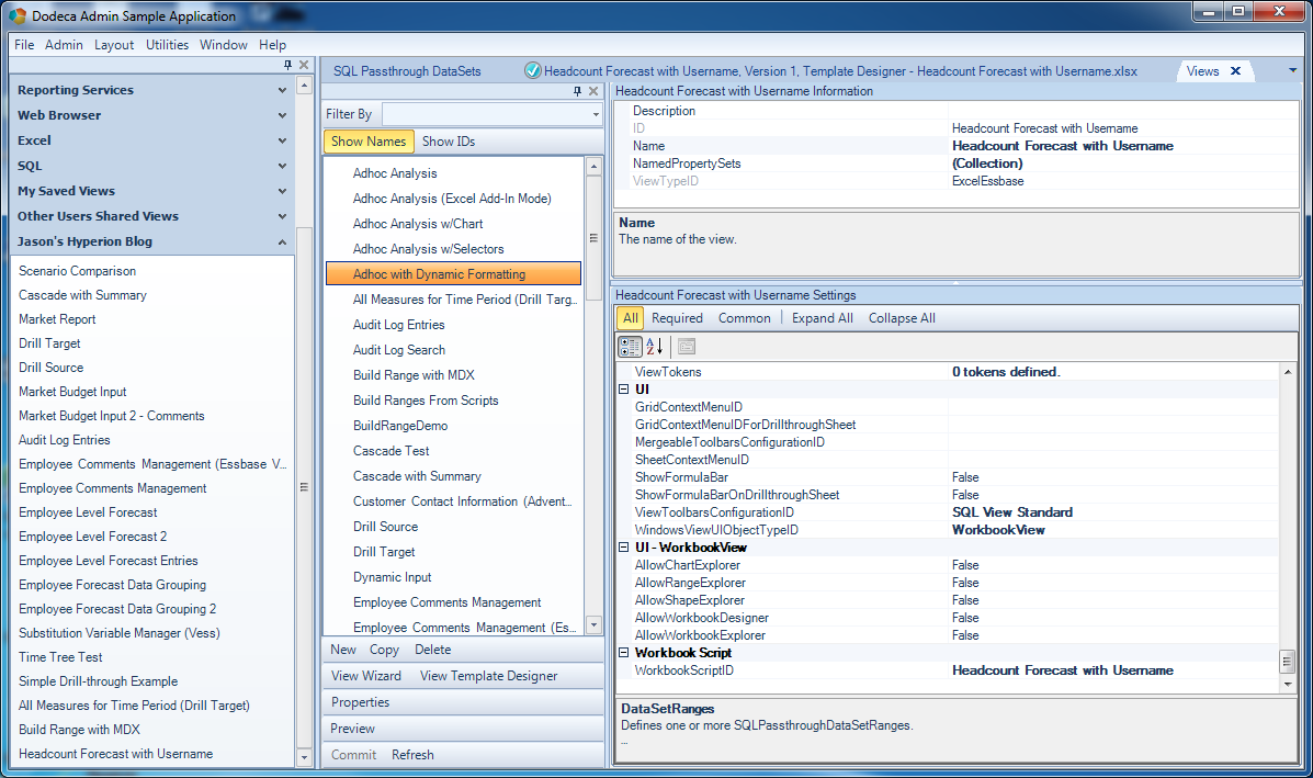
Some of the view properties on the headcount forecast view

Some of the view properties on the headcount forecast view

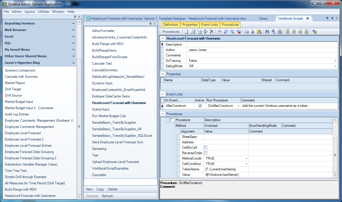
The main thing I want to make sure to show is that there’s a new Workbook Script for this view (as seen in the last row of the view properties). I’m going to jump over to editing this WBS and to do this I can just right click where it says WorkbookScriptID and jump directly to the editor:

Workbook Script for adding a token to the view dynamically

Workbook Script for adding a token to the view dynamically

In the above screenshot, there’s a lot going on, but this shot shows us everything we need to know about the workbook script that I created ahead of time. Remember, the goal of the script is is to be run when the view is built so that we can dynamically create a token to use in the SQL. In the right side of the screenshot, towards the middle, you can see that when the even AfterConstruct is fired, we want to run this procedure.

As for the procedure itself, it’s very simple. I’m using the AddToken WBS method and a specific overload (think version) called View. This method is specifically designed for the use case we have here: to add a token to the view (which we can then use in the SQL Passthrough DataSet or whatever). In the last two rows of the method configuration, I have set the TokenName to [T.CurrentUserName]. Lastly, the value for this token will be set using the @WindowsUserName function. This WBS function (denoted by the @ symbol) is one of the many functions available to us in the WBS language. This particular function  evaluates to the current Windows username. There are actually a couple of related functions related to the current user name (such as the current authenticated user, the current logged in Essbase user, etc.), but for this example, this one will work just fine.

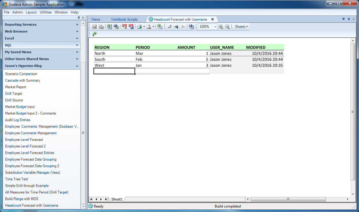
Now when the view is opened, this WBS will run and add the token to the view that we can then reference in the SQL Passthrough DataSet. To now show this all in action, here’s the built view:

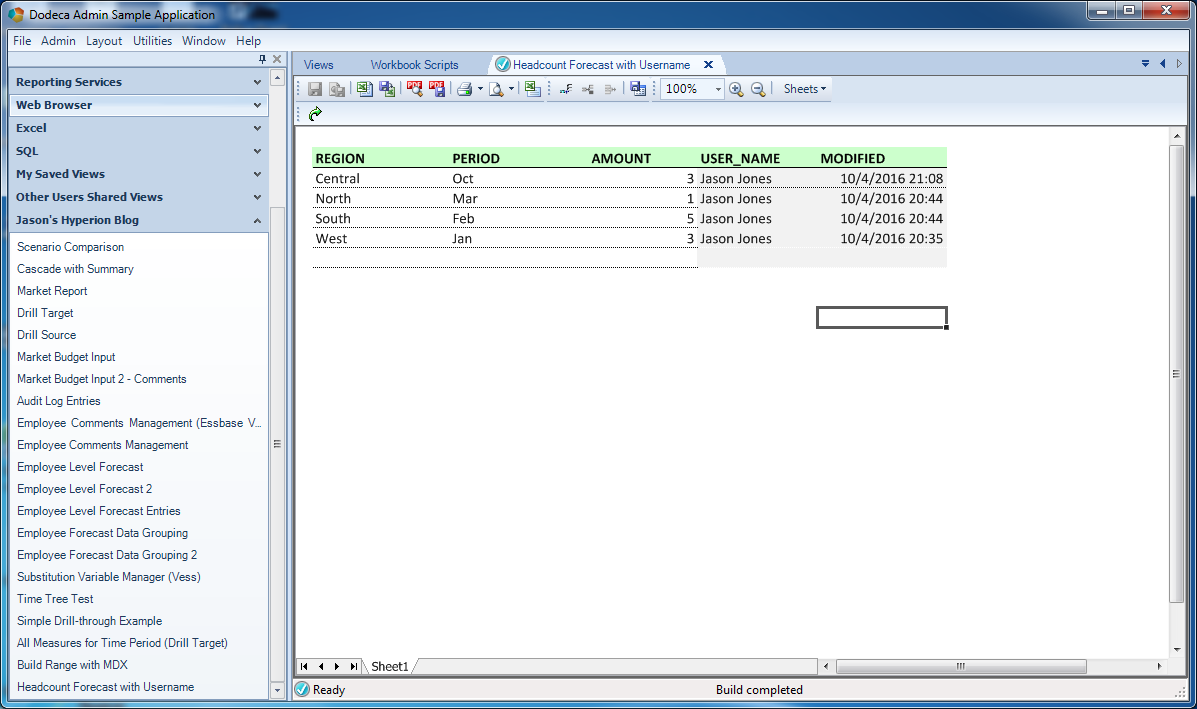
The built view

The built view

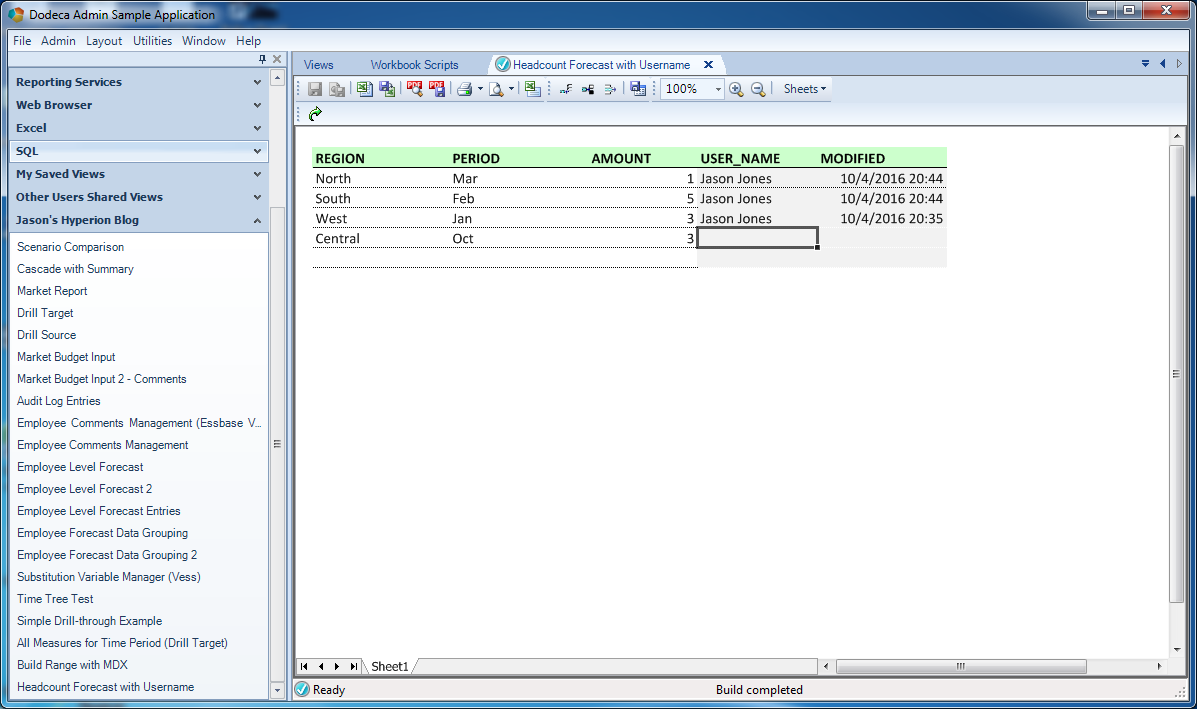
Now let’s type in data for a new row:

Testing the view by typing in a new region, period, and amount

Testing the view by typing in a new region, period, and amount

Note that I didn’t (can’t) enter data for the USER_NAME or MODIFIED columns. And now when I hit the save data button:

The view after saving the data, with the additional columns populated

The view after saving the data, with the additional columns populated

Tada! In my case my Windows user name is “Jason Jones”. The current timestamp was also inserted into the table, as per my SQL definition.

Conclusion

I hope you enjoyed this cross-functional example. It’s a very practical and commonly used technique in the world of Dodeca. To the extent that the layout of a spreadsheet is Dodeca’s declarative side, WBS is the procedural side, and often times it’s the glue (magic glue!) that ties everything together and gives us the power to address the multitude of one-offs that so often need to be accommodated in the enterprise world.

Dodeca Techniques: Dynamic Rolling Quarters

It’s very common to want to perform reporting with a rolling time period. For example, given a particular month chosen by the user, we’d like to display the 4 or 12 or however many previous months to it. We might be given a particular quarter and want to show the previous 4 quarters.

Achieving such dynamic reporting can be tricky in some tools or lead to a less than ideal user experience, but this type of layout can be achieved easily in Dodeca, without having to write any code (although we will use some Excel formulas).

The technique itself is pretty simple, as I will describe in a moment. But I also want to comment on the general technique, since it applies to so many different Dodeca reports. The way that we can easily build this report type has to do with the nature of using a spreadsheet as the basis of the report in the first place.

In Dodeca, we have extreme control over a very methodical report build sequence. The simplest Essbase retrieve we could lay out would be a normal Essbase retrieval grid (members from each dimension, laid out properly). We can then elaborate on this and tokenize various cells in the retrieval grid so that the user selection is placed in for certain cells (such as the time period), and then the grid is retrieved. If we want, we can dynamically build the contents of the grid (such as running an MDX script to retrieve dimension properties). More specific to this case, however, is that we can use use Excel formulas in the cells that participate in the retrieve.

As a simple example, consider a report where the user chooses a year such as FY16. If we want the report to always show the year the user chose, plus the previous year, then we could just write a formula for the column next it, such as ="FY" & RIGHT(A1, 2) + 1. At runtime, Dodeca drops the value from the selector in, and in the case of FY16, our formula will evaluate to FY17, then Dodeca performs the retrieve. Using an elaboration on this technique, we can easily calculate the rolling quarters to show on a report.

Check out this report template:

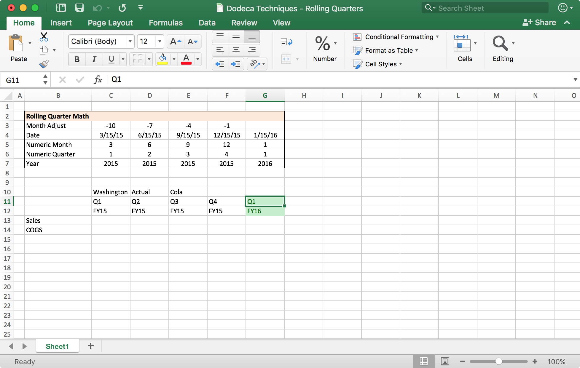
A simple Dodeca template that calculates rolling quarters

A simple Dodeca template that calculates rolling quarters

In this report, I will have two selectors that will fill in the green cells. The user will choose a quarter and a year. The four columns to the left of the green cells are calculated dynamically. The upper area in this sheet is my “work area” that will actually just be hidden when the report is built. For a real world report I would probably have condensed the formulas down a bit, but it won’t affect performance.

Let’s take a look at all of the formulas (again, keep in mind this is just pure Excel, nothing specific to Dodeca), to see what’s going on before walking through it:

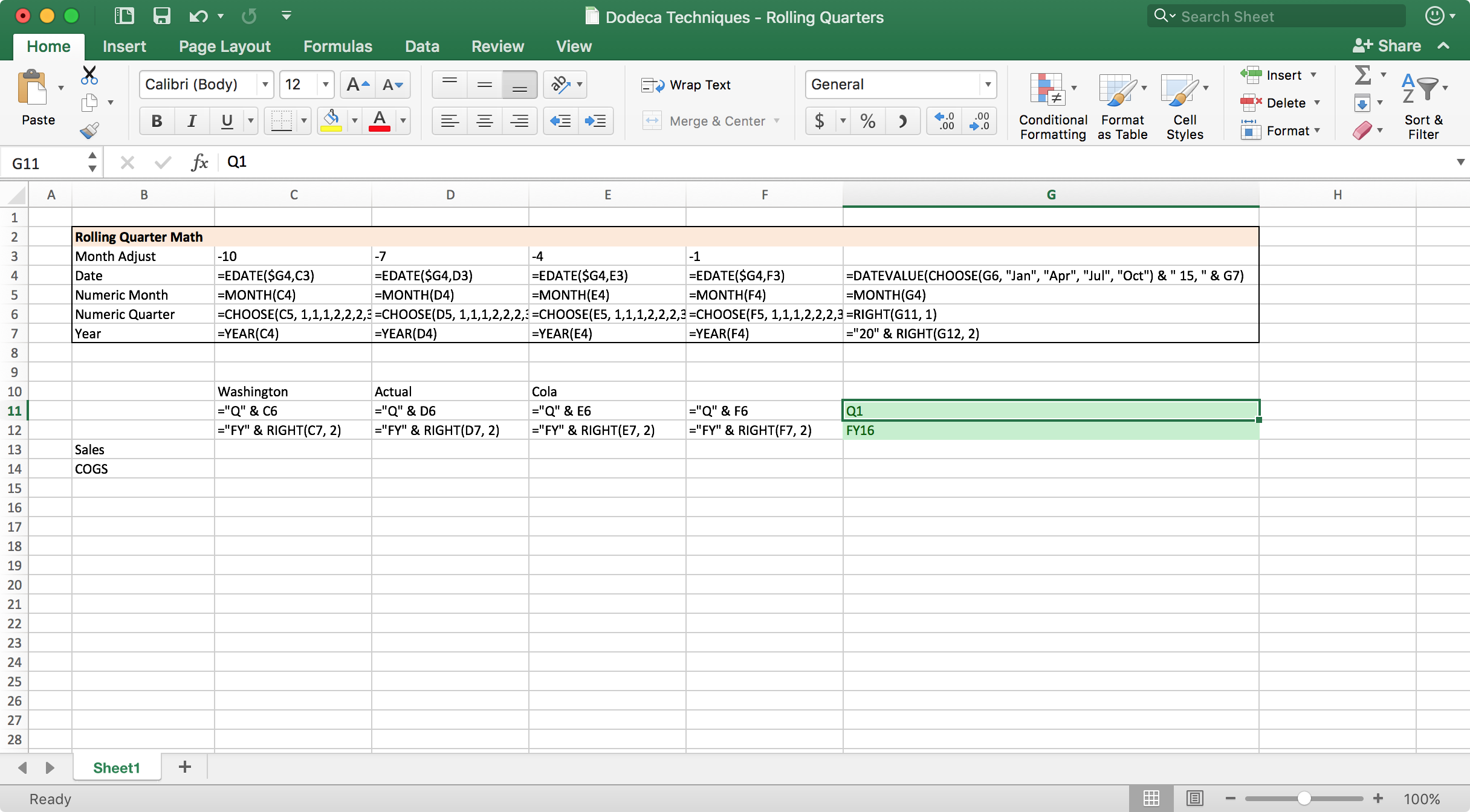
Simple Dodeca template with formula display turned on

Simple Dodeca template with formula display turned on

In sequence:

  1. The numeric quarter is derived from the user selected quarter. Over in cell G6, This is as simple as a =RIGHT(G11, 1). Q4 gets turned in to 4, Q1 turns in to 1, and so on.
  2. The quarter number is “mapped” to a month name using the CHOOSE function in Excel, then converted to a date using DATEVALUE. This is the formula in cell G4: =DATEVALUE(CHOOSE(G6, "Jan", "Apr", "Jul", "Oct") & " 15, " & G7). The CHOOSE function is really, really, useful and powerful in this context.
  3. We extract the numeric month in G5 using =MONTH(G4)
  4. Calculate the year, either using the =YEAR function or building it with ="20" & RIGHT(G12, 2), depending on which column
  5. Up in row 3, notice that we have a “month adjust” value. For the columns to the left of the initial date column, we use =EDATE to calculate the adjusted date based on the original date we calculated
  6. With the numeric month and year in hand, the formula for the cells in our actual Essbase retrieve grid are very simple now: for quarters, concatenate “Q” and the quarter number, and for years, concatenate “FY” and the two digit year.

Again, what happens with the grid is that the user makes a selection for the quarter and the year, we use Excel formulas to calculated previous quarter/year values (by way of converting to a date and using Excel date functions to do the “hard” work” for us), then build Essbase member names in the retrieve grid. That’s it. As I said, this general technique is applicable in many, many use cases, and not just for dates (although it’s particularly effective with dates).


Oracle Open World 2016 Recap

As I mentioned a week or so ago, I made a last minute appearance at Oracle Open World this year. It was my first time attending and presenting at OOW. I actually didn’t catch too much of the conference as I only flew in on Wednesday and flew out on Thursday. Nevertheless, I had a bit of a whirlwind experience, but a very good one. While I hadn’t planned on it (I’m more of a Kscope guy), I am now looking forward to attending Open World next year.

As for the presentation I was part of, I think it went pretty well. Many thanks to Gabby Rubin of Oracle for coming up with the idea for the presentation and facilitating it. The presentation was on “Essbase Tools and Toys” and was meant to highlight, at a high level, some of the interesting things that folks such as myself are doing that involve the Essbase APIs or otherwise work with Essbase. The presentation discussed items created by me, Tim Tow, and Harry Gates. Additionally, Kumar Ramaiyer (also from Oracle) talked a bit about what’s coming with Essbase Cloud Service (EssCS).

I talked about several tools I have created over the years and I think it was the first time I’d really tried to convey an incredibly succinct business reason for why each of the tools exist. So by way of a recap, I wanted to go over those tools here for those that are interested.

In total, I talked about these tools:

All of the tools with the exception of Vess can be downloaded by finding the appropriate page under Projects in the menu for this website. Additionally, there were a few questions and answers that came up (Drillbridge!) that I fielded.

Cubedata

Cubedata is a tool that generates large (or small) quantities of data that can be loaded up to a cube and help test performance. The performance being tested can be the load speed, calc speed, gauging how big the database will be/get, and looking for perhaps better dense/sparse settings, among other settings that can be tweaked.

I created this tool because I couldn’t always work with production (sensitive) data in test, or I wanted to get a more comprehensive feel for how a cube would perform over the years. Automation, calc, and query performance have always been incredibly important to me. Many of the cubes I have designed have withstood the test of time and have been performing very diligently over the years, sometimes with very few changes needing or having been made. The test files generated with Cubedata played no small part in the development of some of these solutions.

In order to use Cubedata, all you need to do is specify lists of member names in some input files (one per line), then optionally pass some other parameters to this command line utility, such as the maximum number of data points to create, what range the values should between, and so on. Cubedata will take are of the rest. I have used to to generate in excess of 50GB of input data.

For bonus points you might even use the Applied OLAP Next Generation Outline Extractor to pull members from your outlines, then feed those in to Cubedata.

Camshaft

Camshaft runs an MDX query against an Essbase cube, then outputs the results to a text file. Many people use MaxL to run MDX queries and feed the results into a cube using a load rule. The bummer about this approach has traditionally been that MaxL puts a lot of junk on the output, so you end up using your load rule as a mini-ETL engine to parse out headers and other junk.

Modern versions of MaxL provide a little more flexibility for MDX output, as blogged about by Gary Crisci. That said, Camshaft gives you a lot of control over the output, and more importantly, keeps the output pretty clean.

Among other options, you can tell Camshaft how to round numbers, whether to show a header or not, how to indent/combine tuples, and more. For people with automation that needs to run an MDX script and load the results somewhere else (to a cube or SQL or otherwise), Camshaft can fit very neatly into the automation sequence and clean things up. Additionally, Camshaft is contained in a single Java JAR file that can be run with the java -jar command (no ugly classpath stuff to worry about!), so dropping it in to an automation sequence is pretty clean.

Vess

Vess is a relative newcomer to the stable of tools and at this stage is still “highly experimental” as I like to say (put another way, it’s fragile. Or ornery. Probably both.

Put simply, Vess is a JDBC driver for Essbase (the name is derived from “Virtual Essbase JDBC driver”). Vess presents a relational facade to Essbase. In a lot of ways, this is like pugging a round peg in a square hold (more relevantly or UML/Visio-ish might be it’s like trying to turn a cube into a cylinder). Vess “models” the Essbase server as a bunch of relational tables. For example, the substitution variables on a server are available in a table with columns such as APPLICATION, DATABASE, NAME, and VALUE.

Vess also models the outline data as a table (similar to the output from the ODI RKM for Essbase or from the Outline Extractor) and the data in a cube itself. You can actually do a normal SQL INSERT to the Vess data table and Vess will load that data into the corresponding cube. Perhaps more usefully, Vess even lets you get at the data in a cube itself via a SQL query.

This opens up a lot of interesting possibilities – such as being able to drop the Vess driver into any tool that works with JDBC, and have instant access to Essbase data. For example, this could mean dropping the driver into ODI to perform a data extract/load, into Data Visualizer, or some other tool.

Vess is a hobby right now but I have provided it to several people that want to play with it and provide feedback. I probably wouldn’t use Vess in production right now but nevertheless, to my knowledge there are some intrepid IT risk nightmares using it for certain things.

Hyperpipe

Hyperpipe runs a SQL command against a specified database (using a JDBC driver you provide, such as to Oracle, Microsoft SQL Server, MySQL, or whatever), then takes the results and loads them to a cube you specify. Given properly specified columns, Hyperpipe loads data without the use or need of a load rule.

Jessub

Jessub is one of the earlier tools I threw over the fence to the public domain, and has a very narrow but useful purpose: it provides a rich syntax for generating substitution variables. Jessub was created because while many systems I worked on/improved used fragile or cumbersome hacks to generate and update substitution variables. Additionally, the vast majority of substitution variables that need to be updated via automation have to do with timing of one kind or another: the year, month/period, week, day, and so on. These are often clumsily (read: fragile) generated from an almost indecipherable batch file expression (or worse, updated manually). Jessub makes it easy to specify a way to generate a variable that might be based on the current year/date/time.

Outline Export Parser

The Outline Export Parser is a simple implementation of a reader in Java that can parse the outline export XML files that can be generated from MaxL in contemporary versions of Essbase. Parsing complex XML files might be beyond the reach of several admins that just want some “clean” output (such as just the member names) from such a file, in which case, the Outline Export Parser might be just the right tool, as you can feed in the XML file and it’ll output just the member names (or more if you want), with optional indenting and some other flourishes.

Rejected Record Summary

The Rejected Record Summary program is not very creatively named. It processes a rejected record file such as from a MaxL import, then summarizes the causes of the rejects. It’s useful if you want to setup your automation to perform a data load (from a text file or SQL), capture the rejects, and email them if there’s a problem (in which case, you might want your automation to email the summary file generated from this program).

Questions & Answers

The audience had a few questions regarding the things I talked about. From memory, here’s some of the things that were asked:

What’s up with Drillbridge?

The short version is this (more coming in the near future!): Drillbridge was acquired by Applied OLAP back in March of this year. It’s existing customers are continuing to receive support. The free edition of Drillbridge continues to live on as Drillbridge Community Edition. This version has always been and will stay free for companies to use as they wish, although it does not come with support or several features in the licensed version of Drillbridge. The licensed version of Drillbridge is now Drillbridge Plus. Drillbridge Plus comes with support from Applied OLAP, and many additional features over the free edition, including advanced reporting types, multi-report drilling, automation integration, report caching/paging, and more.

What’s the performance like with Camshaft?

The performance of Camshaft is essentially determined by how fast Essbase can serve up the MDX query that you run. If the query takes 30 seconds, then the Camshaft runtime will likely be about 31 seconds. Internally, Camshaft just uses the Essbase Java API to run the MDX query.

What’s the performance like with Vess?

Vess is a different story, performance-wise, than Camshaft. Vess (at the moment) doesn’t use MDX to facilitate data retrieves and queries. Rather, it uses the Essbase grid API along with a little magic to try and come up with the data it needs in the most performant way possible. In short, it’s highly variable. Sometimes it’s super fast, sometimes… not so much.

TBC Files for Bankruptcy

After years of declining and inconsistent revenue, the multi-state beverage company TBC has filed for bankruptcy. TBC was known for carrying an eclectic, if antiquated, selection of products that didn’t seem to resonate with modern consumers.

A vice president at TBC for the last 15 years, Richard Doyle, found out that his last day would be at the end of September. “Our products just don’t seem to resonate with the young, hip crowd,” said the forlorn executive, with a wistful look on his face (they don’t seem to resonate with the older crowd either, but I digress). “Kids these days are drinking their fancy this and that, grande double pumpkin bullshit or whatever.”

TBC’s motley assortment of beverages from yesteryear included such unloved profit killers as Birch Beer, Dark Cream, and Strawberry Fruit Soda. The last time TBC introduced a new product to market was 20 years ago, in 1996.

To many, the news of TBC’s impending demise was hardly unexpected. While TBC’s competitors invested heavily in information technology over the years, TBC was known as something of a Luddite in the often ruthless beverage industry, seemingly guided more by whim and gut feeling than data.

Doyle continued in a tone that belied the fact that his company had announced an imminent bankruptcy, perhaps more gambler than executive, “Sarsparilla is going to be huge this year. I just know it. Game changer.”

In recent years, TBC Executives seemed to relent slightly on their general aversion to technology. The anemic IT department hired consultants to develop a system that could more robustly analyze expenses and profitability.

One of the consultants on the implementation effort agreed to speak on condition of anonymity. “We built a good system for them. Profit per ounce, by state, by product, all that fun stuff.” The consultant paused for a moment, then continued, “We [consultants] don’t usually pay much attention to the particular numbers, you know? We just rack and stack cubes, make sure it all ties out. But we couldn’t help but look at their numbers and think, ‘Wow! how are these guys still in business?'”

Confronted with a recent sales report from the new system, Doyle still looked incredulous. “In hindsight, perhaps we should have seen it coming,” he mentioned, almost more of a question than a statement.

Sarsparilla is not, in fact, huge this year.

Camshaft (Essbase MDX query tool) 1.0.2 released

Apparently I’m having quite the productive Friday, what with showing how easy it is to setup drill-through with Dodeca and that I’m heading to Oracle Open World 2017 to contribute to a presentation on cool Essbase tools.

To these articles I’ll add that I just released a Camshaft point release. This release has a couple of fixes and enhancements. Thanks to André Märki and others for providing feedback.

This version of Camshaft fixes an issue where some data with many digits after the decimal would be rendered in scientific notation. Along with this fix I have added a new command-line switch, --maximum-fraction-digits (used on the command-line such as --maximum-fraction-digits=2) to set the max number of digits to render after a decimal.

Additionally, there was a bug with running a query from a file that is now fixed. You can now specify something like --query=somefile.mdx and Camshaft will look for the given file. If found, it’ll read its entire contents for an MDX query, then execute that. This option can help make command invocations with big gnarly MDX queries a little easier to manage.

Please keep that feedback coming and I’ll add enhancements/fixes to the best of my ability. I have some interesting Camshaft news coming in the near future that some people will really like!

As always the latest Camshaft documentation and download can be found linked from the Camshaft page.