jason w. jones

I’m putting together a simple Dodeca view that shows information from Dodeca’s data audit log tables. One of Dodeca’s really nice Essbase-specific functionalities is that it logs all user inputted changes to Essbase data. This comes in handy for many organizations so they are able to tell when something changed, what changed, who changed it, and what the old value is. Because the same tables are used for every single cube in the system and every cube can have different dimensionality, Dodeca uses a flexible table structure to record all of the dimension names and members that changed. A naive query against these tables will give you multiple rows for the same data point (one for each member in the POV), but I wanted something quick and easy to consolidate to a single row per data item changed.

Most of my own Dodeca servers use MySQL for the repository database (although it’s common to use SQL Server, Oracle, DB2, and others). I discovered a really great MySQL-specific function called GROUP_CONCAT that is able to join fields from multiple rows, and it works great. Here’s my Data Audit Log query:

SELECT 
    AUDITLOG.SERVER,
    AUDITLOG.APPLICATION,
    AUDITLOG.CUBE,
    AUDITLOG.USER_ID,
    AUDITLOG.CREATED_DATE,
    GROUP_CONCAT(DP.MEMBER SEPARATOR ', ') AS MEMBER_NAMES,
    GROUP_CONCAT(DP.ALIAS SEPARATOR ', ') AS ALIASES,
    IFNULL(ITEMS.OLD_VALUE, '#Missing') AS OLD_VALUE,
    ITEMS.NEW_VALUE
FROM 
    DATA_AUDIT_LOG_DATAPOINTS DP, 
    DATA_AUDIT_LOG_ITEMS ITEMS, 
    DATA_AUDIT_LOG AUDITLOG
WHERE 
    DP.AUDIT_LOG_ITEM_NUMBER = ITEMS.AUDIT_LOG_ITEM_NUMBER AND
    ITEMS.AUDIT_LOG_RECORD_NUMBER = AUDITLOG.AUDIT_LOG_RECORD_NUMBER
GROUP BY
    ITEMS.AUDIT_LOG_ITEM_NUMBER
ORDER BY
    CREATED_DATE DESC

And here’s a view from a SQL tool:

I went ahead and used the concatenation function twice – once for the regular member names, and again for the aliases. Not every member of every intersection has an alias, but fortunately the function handles it just fine. So now I have everything on one line exactly like I wanted.

Oftentimes when I am demonstrating or teaching aspects of Dodeca to people, they are amazed at the sheer number of options and configurations that are available on a view. Fortunately, I am able to tell them that yes, there are many, many options – and they are there if you need or want them, but they won’t get in your way. The defaults are very sensible and getting a basic Essbase-based Dodeca view running is incredibly easy.

Another thing to keep in mind is that for the most part, the extreme amount of options and flexibility we have on a single view is often available to us in lieu of code. So, tasks that typically required some non-trivial amount of VBA code are now completely code free. When we need some advanced functionality that isn’t available out of the box, we can use Workbook Scripts, which is an event-driven scripting technology that is particularly well suited to working with spreadsheets and the data contained in them.

That all said, today I want to walk through a bit of a cross-functional example that starts with a very typical Dodeca view based on an Essbase retrieve range, then enhance it to give our users the ability to zoom in on the different time periods in the view without having to rebuild the view. So we’re going to blur the line a bit between static and dynamic reports, and our users are going to enjoy some additional flexibility and convenience with regard to their reporting (and keeping users happy is always a good thing, right?).

Imagine the following fairly typical view based on Essbase data:

In the preceding screenshot, you can see that we have a single retrieve range from Essbase with Scenario, Years, and Time on the axes. As with many views in Dodeca, since we can put the retrieve(s) anywhere we want and add convenience formatting, we have the report title, location, and selected department in the upper left corner.

Also note that the row and column headers and gridlines have been turned off. This is easily accomplished via setting a couple of options on the view configuration. For reports like this where the headers don’t really add much, it can really clean things up.

To get a sense of what the Dodeca template looks like, however, let’s go to the view template designer and turn on row and column headers and unhide any hidden rows:

Things are a little more interesting here. Notice that column A is a “template column” that was previously hidden, and row 6 was also previously hidden. This is a very typical technique where the contents of the row are needed to perform the Essbase retrieve, but we don’t actually want to show them.

Template Columns & Template Rows

I’ll get to the notion of template columns and template rows in more depth later in this article, but as a brief aside, I want to explain where we’re headed and what’s going on. As the name might suggest, a template column (or row) is often used as a prototype for copy and paste or other grid expansion operations, particularly when there is a dynamic number of rows to be built. Several facilities in Dodeca can be configured to look to a template, such as a defined range with an arbitrary number of cells, and essentially copy it for new rows/columns that are being generated. This allows us to easily style up dynamic content with the exact style, cell formulae, spacing, and other attributes that we want, without having to resort to code or other shenanigans.

Templates are not limited to a single row/column, either. They are frequently wider/longer, allowing us to easily generate dynamic ranges with complex formulae and other features. In this case we are just going to use a single column as the template.

The last thing I want to point out about row and column templates is that you will often find them above or to the left of the content that is going to dynamically grow. For example, in the grid above, the content is going to possibly grow to include more columns, so I have the column template to the left of all of that. This makes my life a little easier since I know that the location of the column template isn’t going to move around on me. Because rows and columns that we hide on the view template will stay hidden (but are still completely functional), I can just hide the template and not have to worry about it.

Now Back to Our Template Layout

Just to make things clear about the Essbase retrieve range, here it is exactly on the template (Note the defined name of Ess.Retrieve.Range.1):

Again, the top row with the POV members is going to be hidden because we are going to format those more nicely in the upper left. Our column template also gets a name and defined area:

The column template isn’t going to have Essbase data retrieved directly in to it, as you’ll see later, it’s purely for formatting purposes. Notice that it also has a defined name of Column.Template (so that we can refer to it easily in Workbook Scripts and other places that might need it).

That’s actually just about all we need for the view template itself. The rest of what we need to configure is the view properties and a workbook script to help with some of the dynamic formatting that we want.

There are a few options that we’re gong to use on this report that I haven’t talked about before, but are going to come in very handy. Check out the options I’m using in my Behavior – Essbase category:

Of note, I have AllowEssbaseOperationsOnRetrieveRange set to True and AutoAddRetrieveSubRanges also set to True. The first option is where I can tell Dodeca that yes, I want users to be able to interact with a given Essbase grid on the build view. By default this is off (we’re turning this on so that users can double click on a time period to expand out to the children time periods on the built view. I just need a couple of other options set to round things out:

Besides some of the UI things I set, the main options to note are the Member Drillthrough options. This is where I can configure the exact behavior for double clicking on a member on the grid. Nicely enough, I can even specify the exact dimensions that a member can drill into. Because I only want to let the Periods dimension be expandable (and not others), I simply specify that dimension name here and now the user will only be able to expand that dimension.

Our New Best Friend, AutoAddRetrieveSubRanges

Next, let’s talk about this AutoAddRetrieveSubRanges option. This is a really, really fantastic option because of all the amazing utility and convenience it can provide to us. What this option does, is that when it’s set, Dodeca will retrieve Essbase data, and then automatically create new subranges (defined names) within the overall retrieve range that outline exactly where the rows, columns, POV dimensions, and data reside.

Think about this for a minute. This is particularly poignant in the context of what I might call “Configuration over code”. Let’s say that we weren’t using Dodeca for this report. Let’s say that we had an Excel book that we wanted to automate with some VBA. So we write some code to connect, cycle through a range, retrieve from Essbase, format the data, put it in the right cells, clean up the connection, and more. Then maybe we need to write some more code to figure out which axis is which (row/column/POV/data). That’s a lot of code to write. That’s an insane amount of code to write considering that we can have this behavior out of the box with a couple of checkboxes in Dodeca. Just to hammer this home, let’s take a look at the effect of turning this option on for a typical Essbase retrieve.

There are four ranges that are going to be added automatically to the view when it is built. Here’s the range that gets created automatically for the POV members:

And for the column headers:

And for the row headers:

And for the data itself:

Before getting in to the workbook script that is going to tie this all together, I want to show the look we are going for. The report will nominally built to show quarters and the full year value, but we want the user to be able to double click on a quarter and expand the report out (via a quick retrieve to Essbase) to the the months in that quarter – all without having to rebuild the view itself. Double-clicking on Quarter 1 should make the report look like this:

A Little Workbook Script to Tie It All Together

You might be wondering why the automatically generated range names were so important earlier. Well, it has to do with the workbook script that we are adding to this view. You see, one thing that we need to define for ourselves for this blend of static/dynamic view is how the newly drilled members should be formatted. And as it turns out, my requirements for this report are that the color of a header column should be different depending on whether it is a period/month, quarter, or the whole year.

Workbook scripts (WBS) are event driven groups of actions that can be added to a view. In many ways, they are to Dodeca what VBA is to Excel. That said, they are also meant to be more powerful, flexible and maintainable.

In the world of Essbase and Excel programming, there are very many actions and activities that revolve around iterating through rows and columns of cells. Sometimes these activities need to operate on a whole range, sometimes on every individual cell, sometimes it depends. It’s these types of activities where WBS really shine and our automatic named ranges are going to come into play.

As it turns out, the list of columns that we need to dynamically format using the WBS exactly coincides with the column headers range that was automatically added to the Essbase retrieve range.

What I’m going to do now is step through the entire configuration of the workbook script so you get a sense of how they work and some of the features they offer.

Properties

Remember that I wanted to have different colors depending on the level of the time period? Let’s setup properties on the WBS so I can easily configure these. Every WBS can have its own properties, which are basically like constant variables (in the world of programming). In the following screenshot, in the Properties section of the WBS, you can see that I have defined three different properties (ColorLevel0, ColorLevel1, ColorLevel2) and defined them with a particular color each:

Isn’t that kind of interesting, actually? I didn’t have to specify some hexadecimal value or anything – WBS inherently knows about a property type that happens to be a color, and it even pops up a color picker dialog when we want to configure them. Nice.

Event Links

Workbook Scripts are event-driven. Essentially this means that we can attach behavior to wherever we need it in the view lifecycle. For example, for this script I need to put custom behavior in for when the workbook opens (to set some colors), and then some behavior that fires any time that a retrieve operation is performed in the book (e.g., when the user double clicks on a time period).

You can see the two events I am using in the previous screenshot. I have procedures specified for the AfterSheetRetrieveOperation and AfterWorkbookOpen events, that will execute the methods OnAfterSheetRetrieve and OnAfterWorkbookOpen respectively.

Procedures

This is the last thing we need to make it all work, and this is really the crux of the script, where we actually do something. Let’s first look at the OnAfterWorkbookOpen procedure. We’re going to use this event to initialize color values in the workbook. You see, one of the ways that Excel works with colors is that there can be a fixed palette where an integer refers to a specific color (it’s also possible to create colors arbitrarily, but in this example it’s actually more useful to refer to colors by index). Referring to colors by index is going to be really useful for us because we are actually going to just take the level of an Essbase member (0 = Month, 1 = Quarter, 2 = Total) and use it to figure out the right color. We definitely don’t want to use the default color palette because this would have us end up with red, green, and blue.

What we can do, however, is set arbitrary colors for indexes. Therefore, when the workbook opens, we want three methods to fire to set a color index for each of the variables we defined earlier. In the following screenshot, notice the three SetColor methods. You can ignore the first seven rows of the method (the rows containing SpecifySheetBy, SheetSpec, Address, so on). These are part of every WBS method but oftentimes we don’t need to set them (we’re going to use them in a moment for the other methods, though, so stay tuned).

The only configuration for the SetColor method we need to concern ourselves with right now is the Color and the Index. Each SetColor method is going to set a different color index (1, 2, and 3) for one of the three color level properties we set. The @PVal (property value) function references the respective property value for us.

Note that for technical reasons I decided that the color index to change for a given level would be that level plus one. So the color index for members at level 0 is 1, level 1 is 2, and level 2 is color index 3.

Where the Magic Happens

We only need to set the colors once when the workbook opens (as opposed to after every grid operation or more often). Now we can turn our attention to the final piece of the puzzle, which is where we are going to dynamically format the newly expanded columns, using a color index we set, processing across a range that is automatically added to the sheet for us, dynamically formatting things based on our column template.

There are just two methods that make up our OnAfterSheetRetrieve procedure. The first is to set the cell background color. This is the background color for the header cell in a given column and is dynamic based on the level of the member. The second method is where we copy the column template over.

Set the Column Background Color Dynamically

Let’s walk through the method to format the column header color. Unlike our earlier SetColor operations, we are going to adjust some of the base method properties. We’re going to specify the Address and CellByCell options:

The Address value determines what range the method operates on. Turning on CellByCell means that the method will be called iterative for each cell. Again, I mentioned this earlier but it bears repeating this. This configuration is all in lieu of VBA or other code. Another way to look at it this is that what would typically be many nested FOR loops and conditions in code is now just a couple of simple configurations that we can optionally use.

That all said, the real magic in this method is the FillColor. While we could specify an arbitrary color here, we are actually going to make this dynamic based on the level of the member being processed. We can accomplish that with the following code:

=@MbrLevel(@ValueText(@ACell())) + 1

The function names preceded with @ are all native WBS functions. They typically offer us very handy behavior when it comes to processing things with WBS methods. This formula will take the text value of the active cell, then find out its Essbase member level, then add 1 to it. This lines up with one of the color palette index values we set earlier.

If I wanted to translate the entire method to English, I might do it as the following: please process over every single cell in the range Ess.ColumnHeader.Range.1, then set the fill color to the color palette index that is the level of that member name plus 1.

Copying in the Template Column

Now that we have the background cell color set, we can turn our attention to copying in the template column. We mostly just want this for the formatting, and indeed, we’re going to only copy the format from the template column. This will bring in the numeric formatting we want background color, and borders.

Let’s take a look at the method definition:

Copying the template range based on the current cellThis time we are using the CopyRange method. As with before, we are going to process over each cell in the column header range, cell-by-cell. The CopyRange method has a few things to set: the source range to copy (our defined range Column.Template), and a paste type (Formats only, as opposed to values or other types of pastes).

The PasteRange is the most crucial element in this particular method. You may notice from the screenshot that it’s a bit of a doozy. I won’t explore it in exhaustive detail, but I want to point out that basically what’s going on is that we are iterating over each cell in the column header, and we need to specify the column range to paste the formats of the column template into. The address for that column range is therefore based on the address of the current cell, but is below it and has a certain determinable height (i.e., the same height as the column template itself). If you’re interested in the complete explanation of the formula, please contact me and I’ll do a follow up post.

All Together Now

Alright, it took a little while to walk through, but we made it. We built a normal view template based on some Essbase data and selector values (a bread and butter view for Dodeca, if you will) with some light formatting, but then decided that we wanted our users to have a little bit of advanced functionality to dig into one of the dimensions a little further. So we turned on the ability to zoom on members in just a particular dimension, then added some workbook scripting to apply some dynamic formatting for us. Although we had a couple of relatively “dense” expressions in a couple of workbook script methods, it was all pretty logical – and perhaps more importantly, is much more maintainable and less complex than the equivalent VBA would have been.

Now when the user opens up and builds the view for the first time, they get this:

And a simple double click on Quarter 1 will change the report into this:

And that happens all without having to go to a different view or rebuild the report. I hope you found this example with advanced view options and some custom WBS useful, and as always, don’t hesitate to reach out with any questions.

Have you ever wondered what the difference between a JDBC and a JNDI connection is? If you’re familiar with at least one of these, it’s likely that you’re familiar with JDBC (but probably not JNDI).

JDBC connections come up often in the Oracle world (for good reason). It’s a standard model/framework for designing drivers that interact with relational databases. As it pertains to us in the Hyperion, Dodeca (and even Drillbridge!) world is that we often define connections in terms of specifying JDBC parameters. This typically means a driver class name (like com.mysql.jdbc.Driver for a MySQL driver), a JDBC URL (a URL specifying a server and optionally a database/schema and other parameters), and credentials (username/password). So if you’ve poked around in your infrastructure much at all, there’s a good chance that you’ve come across a JDBC connection.

You may have even come across something called JNDI and even vaguely known it was sort of an alternate way to configure a connection but never really had to bother with it. I’ll spare you the acronym details, but think of JNDI as a way of organizing database connections (and other objects actually, but we don’t need to worry about that at the moment) such that instead of our app/system having to know the server name and credentials, it just asks “Hello, can I have the resource that was defined for me with name XYZ?”

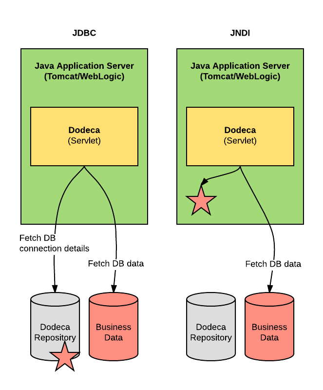
For the application in question, the net result is much the same: a database connection is gained and the database operations are executed as normal. Consider the following diagram that compares these two ways of organizing the database resources, as it pertains to a connection we might want to make from an application such as Dodeca:

In the first, and most common scenario, we have a Dodeca servlet (yellow) sitting inside of a Java Application server (Tomcat in this case). Dodeca talks to its repository and asks for the details for a defined SQL (JDBC) connection (the red star, representing the connection details stored in the repository along with everything else). Given those credentials, Dodeca (the app) then makes a connection to that particular database (the red cylinder) and does whatever with it (executes a SQL query such as SELECT or INSERT). Again, this is the typical configuration scenario.

The nuance to keep in mind here is that at some point in time, the connection details, meaning the JDBC parameters such as driver class, URL, username, and password, had been specified and entered in to the app (Dodeca) and stored in it’s repository.

But what if, for some policy/organizational/legal/technical reason, the powers that be at a given organization decided they didn’t want to have these configuration details in the repository? Maybe it’s due to separation of duties, SOX compliance, or some other reason. But they might say, “You know what? We’ll define the connection for your system and you can grab a connection via its name, but won’t have access to the username/password?”. This would be an organizational situation where JNDI could be appropriate.

With JNDI, the configuration details for the database are now stored in the container itself (as noted by the red star in the green application server/container). So now, the app (Dodeca) would ask it’s parent container “Hey, can I have the connection named XYZ?” and then connect to the proper database (red cylinder) without having to know the driver, URL, username, or password.

In this case, the connection in Dodeca (or whatever the end system is) is now defined differently (and a bit more simply) as in the following:

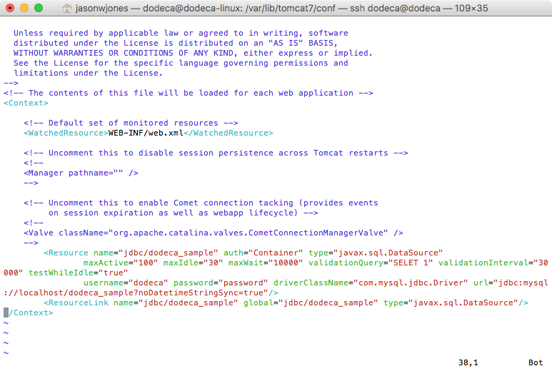
Note the “DataSource” parameter with the JNDI resource name – and node that the JDBC section is empty, along with the Security section. Each container, be it Tomcat, WebLogic, or whatever, has its own way for defining JNDI resources, but in Tomcat, it might look like the following:

The preceding is a screenshot from a configuration file for Tomcat that defines resources. The entire Resource tag is used to define the connection by giving it a name, specifying some parameters, the driver class, and any pertinent configuration details.

As I mentioned, at the end of the day, the end result is much the same: the application gets a connection to a database one way or another and operations are executed as normal. I find that the reason for using a JNDI connection is typically less technical than organizational. Specifying resources this way can also be useful if you want to let the target app use the same configuration between development/QA/environments, although given the way that Dodeca organizes connections, it isn’t an issue.

This post might alternately be titled, “So you’re really stubborn and wasted a couple of hours messing with the Essbase Java API”, or something. I was in a discussion the other day and asked about the ability to run an application-level calc script.

Well, back up, actually. Did you know that calc scripts can exist at the application level in Essbase? For a very long time, Essbase has had this notion of applications and databases (with databases often just being called cubes), such that there is usually one database/cube inside of an application, but there can technically be more (at least in the case of BSO). It’s almost always the best practice to have just one cube to an application. This is largely for technical reasons.

That said, while objects like load rules and calc scripts typically exist within the folder for a given cube, they can technically be located inside of the application itself. In theory you might want to have a calculation script that is applicable to multiple cubes in an app, and would want to centralize it in the application. Here’s a screenshot of the Sample app showing that there is, indeed, a calculation script located in it (that I have placed there);

The most generous thing I can think to say about application-level objects like calc scripts and load rules is that they are essentially a vestigial organizational paradigm from yesteryear. While Oracle hasn’t gone out of their way to prohibit their use, they haven’t gotten any love (nor would they necessarily warrant it). You can’t create them directly in EAS (you can copy an existing script from a cube, which is what I did for the above screenshot). You can’t run them from Smart View. I don’t believe there is a way to grant access to them from Shared Services (cube level calcs, no problem).

You can technically run them using MaxL and run them from EAS.

What you can’t do, however, is run them using the Essbase Java API. That’s where this post comes in. I was really wondering if it was possible to run an app-level calc using the the Java API. But there’s no method for it. The typical method you’d use is calculate() on an IEssCube interface. But there’s no equivalent method for an IEssOlapApplication. Usually you pass a calc script name to the calculate() method, but you can’t try and trick it with a relative folder path or pass in null or something.

However, the old C API for Essbase could run an app-level calc. It turns out there’s a function there that can take null for the cube parameter and will just assume the calc lives in the app.

Surely, I thought, there’s a way to make this happen or maybe trick the Java API into doing my bidding for me. I thought that maybe if I could get the Essbase Java API to pass a null cube name in for me, I could maybe trick it. I took a look at the bytecode (compiled files in the Essbase Java API) and found that it’d be impossible, actually, to try and supply an arbitrary cube name to the calculation function, because of the way that it reads the cube name from the class itself.

That said, there appears to be a very dirty/hacky way to trick the IEssCube implementation into passing a null value in and getting the underlying C API function to execute the app-level calc.

The trick is to subclass EssCube (the implementing class for IEssCube) and selectively override a couple of methods so that when the calculation method is invoked, it reads our fake cube name of null, then executes the calc.

Anyway, here’s a GitHub Gist with the sample files for tricking the Java API into running an app-level calc. The real trick is to allow for specifying a fake name as well as also overriding the setActive() method that is called internally int the Essbase Java API so that it doesn’t just blow out the fake value we’re supplying.

So, when would you use this? The answer is never. You should never, ever, ever do this. It’s using a private API class (bad!), to facilitate a functionality that is of marginal usefulness in the first place, is rarely used, and isn’t getting much support.

Nevertheless, in some ways it’s an interesting example of being stubborn hacking an API to try and do your bidding when the out of the box functionality isn’t quite sufficient.

Lately I have been working on new materials and demo ware to help show off the power, flexibility, and sophistication of both the Dodeca Spreadsheet Management System and Drillbridge/Drillbridge Plus. I came across a really great Drillbridge mapping example today that I hadn’t specifically solved before, but with a little creativity I was able to write the proper Drillbridge query and get exactly what I wanted.

Consider an Essbase cube with the following dimensions:

• Years: FY15, FY16, etc
• Periods: Periods/Quarters/Months
• Scenario: Actual, Budget
• Departments: balanced hierarchy with four levels
• Location: Total/Division/Store
• Measures: Ragged hierarchy with accounts at level-0

For this post I am going to design a Drillbridge query that maps from this cube back to its related relational data, with the additional wrinkle that we want upper-level drill in several dimensions, including one where the dimension in the cube is represented by two different columns in the source data.

Here’s a screenshot from EAS of what this looks like:

Let’s now turn our attention to the underlying transactional data that we want to drill to:

The upstream transaction data adds a few things that aren’t present in the cube, such as a transaction ID, transaction date, amount, and a memo. In terms of mapping from the cube members to the columns of data, things are fairly straightforward. The Scenario values are exactly the same, so that’s easy. The period is represented numerically as well as with a three-letter month (“Jan”), so that’s easy as well (if we didn’t have the three letter month name in the relational data, we could just easily use a built-in Drillbridge function that converts month names to numbers). The account is also a straight mapping. The division and location are a little interesting, however.

Notice in the cube that each entity/location is made up of its three digit division, a hyphen, and a three digit location number, such as 701-101. This is actually really easy to accommodate in Drillbridge because the Location will be passed in and it’s easy enough to use the substring function to get the first three digits and the last three digits.

Where things get interesting, however, is if we want to provide upper-level drill in the Location dimension. As an example, this is what we might need/want a generated query to look like:

SELECT 
	* 
FROM
	SUPERMARKET_TRANSACTIONS 
WHERE 
	YR = '2014' AND
	PD_NAME IN ('Jan', 'Feb', 'Mar') AND
	SCENARIO = 'Actual' AND
	DEPT IN ('001') AND
	ACCOUNT = '0170100' AND
	(DIVISION, LOCATION) IN (('701', '101'), ('701', '102'))

Note that this code example is for MySQL, the syntax and technique varies a bit for Oracle or Microsoft SQL Server. Pay particular attention to the last line. Remember, in this table, the division and location are separate columns but are derived from a single incoming value or values. In order to properly check for the proper values (in the case of multiple locations) we actually need to verify that a given tuple (such as ('701', '101') of values exists. If the user drills from an upper level member in the Location dimension, you can kind of imagine that multiple level-0 members area going to be processed for Location token, such as 701-101 and 701-102 (to be clear, Drillbridge only handed a single member that was actually drilled on, Drillbridge takes care of figuring out the descendant members, whether it is from Essbase or PBCS).

So, knowing that, we can carefully construct the proper Drillbridge token to generate the query that we need. And here’s what that token expression looks like:

\"('\" + #Location.substring(0, 3) + \"'\" + ', ' + \"'\" + #Location.substring(4) + \"')\"

This looks kind of gnarly, but let me break it down for you. When you drill from upper level members in Drillbridge, Drillbridge gets all of the levef-0 descendants of the drilled member, applies them one at a time to your expression, then joins them all together (such as with a comma) in order to generate the final expression that is dropped in to the query. So first of all, the expression above, when applied to a single incoming member name (like 701-101) will generate this: ('701', '101').

The reason for the backslashes is to escape the double quotes. So from left to right we have this:

• Start with an opening parenthesis followed by a single quote: ('
• Apply the substring function to the value in the #Location variable. Substring is the Java String function of the same name, which is given a starting character (strings start with character 0, and an ending character (exclusive), such that the substring of the incoming value 701-101 will be 701.
• Add on a single quote and, comma, a space, and a single quote: ', '
• Now use substring on the location variable again but this time to get the last three characters, so that 701-101 becomes just 101, for example
• Follow that all with a closing parenthesis: )

Drillbridge will automatically join all of the individual values with commas and surround the whole thing with parentheses. Also note that the reason we are treating the division/location as strings (and quoting them) is because in this case, they are strings (more specifically, they are CHAR(3) columns in this table).

All that said, here’s our final Drillbridge query, complete with turning on drill to bottom for various other tokens:

SELECT * 
FROM
	SUPERMARKET_TRANSACTIONS 
WHERE 
	YR = '{{"name":"Years","expression":"'20' + #Years.substring(2)","sampleValue":"FY14","overflow":"","overflowAt":0,"flags":""}}' AND
	PD_NAME IN {{"name":"Periods","expression":"#Periods","drillToBottom":true,"sampleValue":"Qtr1","overflow":"","overflowAt":0,"flags":""}} AND
	SCENARIO = '{{"name":"Scenario","expression":"#Scenario","sampleValue":"Actual","overflow":"","overflowAt":0,"flags":""}}' AND
	DEPT IN {{"name":"Departments","expression":"#Departments","drillToBottom":true,"sampleValue":"001","overflow":"","overflowAt":0,"flags":""}} AND
	ACCOUNT = '{{"name":"Measures","expression":"#Measures","sampleValue":"0170100","overflow":"","overflowAt":0,"flags":""}}' AND
	(DIVISION, LOCATION) IN {{"name":"Location","expression":"\"('\" + #Location.substring(0, 3) + \"'\" + ', ' + \"'\" + #Location.substring(4) + \"')\"","drillToBottom":true,"sampleValue":"701","quoteMembers":false,"overflow":"","overflowAt":0,"flags":""}}
ORDER BY TRANS_ID

One of the really great features in Drillbridge Plus is the token editor GUI that makes editing token parameters in queries a snap. Here’s a screenshot of editing our kind of complex Location token in the editor:

Back over to the report configuration itself, we also need to make sure to set the Essbase Connection for this Drillbridge report definition, because Drillbridge needs to know which cube to inspect in order to determine what the level-0 members are:

Just for fun, let’s also tweak a couple of the options available on this report type. Of particular interest is that I want dates to be formatted nicely (Smart Formatting) and I want to turn on auto numbering, which will cause a column to be sliced in automatically with the current row number (I could achieve this in SQL but it’s really easy to just turn on the Drillbridge feature):

With all of that configuration out of the way, we are now ready to test things out. Nicely enough, I have defined “sampleValue” parameters for all of the tokens, which means when I go to test the report configuration out, the boxes are all filled in for me. This is one of my favorite features because it saves a ton of time during development:

Of particular interest in this test configuration is that you can see I am drilling on a division (because I want to make sure my upper-level drill is working properly) as well as an upper level time member (Qtr1) so I can also make sure that that’s working. Here are the results of executing the report:

I’d be lying if I said I got this to work on the first try (I always forget a comma or quote somewhere), but here we are, with our auto number column, automatic formatting on the dates and amounts, and more importantly, all of the proper data for all locations under the division we wanted to see. After this, I defined a quick deployment spec (not pictured) to allow for upper level drill in the Location dimension (and others), deployed it to the cube, and fired up Smart View to verify the drill-through to be working.

After quickly getting my ad hoc sheet configured (and using the bright neon lime green to highlight drillable cells), I set things up just right in order to test the same intersection from Smart View (meaning drilling on a quarter and a full division). Here’s the sheet as well as the results of the drill-through request:

Summary

I really enjoyed being able to use Drillbridge to map data from the cube to relational for this non-trivial mapping example. I think this was a really nice, clean approach that retrieved the exact data that we wanted. Another way we could have solved this and kept the Division/Location mapping even simpler would have been to actually just use a view to combine the division and location with a hyphen, then we could compare the values from the Location dimension directly. This technique is often employed when you have control of the target database and you just want to keep your Drillbridge query as simple as possible (as in all tokens are just passed right through with no adjustment). Either approach works just fine, although often there’s no ability (for technical/security reasons) to put in custom views. You can also use an ETL tool to extract out the data you need (and map it in to a format that’s conducive to the cube) but then you are introducing more moving parts and more development effort. One of the reasons so many companies are enjoying Drillbridge is that it keeps the development time (and moving parts) down to a minimum.

Earlier in the week, my archnemesis colleague Cameron Lackpour hosted a guest blog article by Chris Rothermel with a trick for deleting multiple files from PBCS using the epmautomate tool. The basic idea is that you can use the listfiles command to export the list of files to a temporary file, then use some batch scripting to iterate over every line in that file, then call epmautomate to delete the specific file. It’s a good example that will undoubtedly come in useful for many people.

Upon reading the article I thought it would interesting to do the same thing, but using the PBJ library. The PBJ library is an open source, 100% Java library for interacting with PBCS via its REST API. It can easily be dropped in to enterprise Java projects by including its dependency in your Maven configuration file (if you’re so inclined). The PBJ library is also used in at least one major piece of software: it’s the library that allows Drillbridge to perform upper level drill from PBCS to a relational database.

That all said, one of the nice things about having a domain specific library in a high-level language such as Java is that it is sometimes very easy and straightforward to implement functionality that doesn’t come out of the box. This doesn’t make it better than the batch scripting technique, just different.

Here’s the whole code file:

package com.jasonwjones.pbcs.misc;

import com.jasonwjones.pbcs.PbcsClient;
import com.jasonwjones.pbcs.PbcsClientFactory;
import com.jasonwjones.pbcs.TestHarness;
import com.jasonwjones.pbcs.interop.impl.ApplicationSnapshot;

public class DeleteAllFiles extends TestHarness {

	public static void main(String[] args) {
		PbcsClient client = new PbcsClientFactory().createClient(createConnection());
		
		for (ApplicationSnapshot snapshot : client.listFiles()) {
			client.deleteFile(snapshot.getName());
		}
	}

}

Most of this is pretty standard boilerplate Java. You can that after we setup a PbcsClient instance, we can very easily get a list of files (using listFiles()), and then iterate over those. To delete a file, we can use the deleteFile(String filename) method and pass in the actual file name from the “snapshot” object (which also contains a little bit of other information).

That all said, as I’ve written before, the best tool for the job is the one that fits in to your environment the best and is easiest to maintain. If you’re doing much in the way of batch scripting, then epmautomate is probably going to fit into your environment the best. If you’re writing an enterprise app in Java, you’re going to absolutely want to use the PBJ library rather than try and execute shell commands.

I had a need for the Hyperion Parent Inferrer functionality for an internal project I am working on. It didn’t quite do what I needed out of the box so I updated things a bit. As quick background, the Hyperion Parent Inferrer is a simple one-off Java program/library I developed (apparently four years ago, wow) to parse indented data into an explicit parent/child file.

There are a few (apparently rare) cases where this is useful. In my case, I was modeling some hierarchical data and I find the indented format to be much easier on the eyes. Like so:

Time
 Q1
  January
  February
  March
 Q2
  April
  May
  June
 Q3
  July
  August
  September
 Q4
  October
  November
  December

But when it comes time to load in to Essbase, clearly we need something more explicit. The Hyperion Parent Inferrer takes that preceding as input and then outputs something like the following:

,Time
Time,Q1
Q1,January
Q1,February
Q1,March
Time,Q2
Q2,April
Q2,May
Q2,June
Time,Q3
Q3,July
Q3,August
Q3,September
Time,Q4
Q4,October
Q4,November
Q4,December

The program has been enhanced to allow for a custom indentation character (such as tabs), to be able to specify the text rendered when there is no parent (instead of null), and a couple other little cleanups.

Hyperion Parent Inferrer is free, open source (Apache Software License version 2), and can be run as a standalone command-line Java program or as a Java library that can be incorporated into a typical Java program. The updated code is available at the Hyperion Parent Inferrer GitHub page.

For some reason the other day I was thinking “Whatever happened to that renegade members feature?” So I did some digging.

Renegade members, by the way, refers to this concept where instead of a data record being rejected, you can map it to some other member. Other names for this feature might have been “shovel members”, but renegade members sounds cooler. That said, it’s a feature with a cool name but an apparently terrible publicist.

Renegade members were blogged about as early as a few years ago, such as on Cameron’s blog (during the 2013 OpenWorld), in Russian (apparently), and even over at Rittman Mead’s blog (before Mark spent his days trying to get tea kettles to work with the internet, but I digress).

But there’s a a curious lack of information on renegade members since then. There is, however, just enough information on the internet to piece this together. There’s a little documentation about renegade members over on the official documentation. Just as important (for my purposes), there are two methods relating to renegade members that are in the Essbase JAPI Javadoc.

Typically when something is in the JAPI, there is a fair chance that functionality is in EAS as well. And since the renegade member is related to the dimension object (IEssDimension) I went hunting around in EAS for any sort of menu/right-click setting or anything that would let me select the renegade member. It may exist, but I couldn’t find it anywhere. So right now my assumption is that it doesn’t have a GUI to manage it (at least in EAS). Further, there doesn’t seem to be any MaxL syntax to update the renegade member. So that leaves us with literally these two JAPI methods to update things.

A Few Hours Later in Java Land

Not to be deterred by a lack of GUI or commonly accepted form of administering an application, I whipped up a quick and dirty Java app to try and update the renegade members for a given dimension. You won’t be able to compile it and run it out of the box (it relies on some private libraries I’ve developed that aren’t public), but you can check out the code such as it is over on a GitHub project (imaginatively titled Hyperion Renegade Setter) I created.

Basically, it takes a given Essbase connection and a dimension/member, then tries to update that dimension’s renegade member. It also allows for clearing the renegade member. These APIs are little bit touchy but I think I have the sequencing right. Of course, there is absolutely no warranty expressed or implied, so caveat emptor.

Here’s an example of setting the renegade member for the Products dimension:

And an example of clearing it:

Please note that the code here is simulating running on the command-line. I haven’t gone so far as to compile this for the command line and actually run it there, but if you’re dying to do so and don’t want to mess with adapting the source code online, send me an email and I can make available.

Also, sidenote: renegade members are only available on ASO databases, not BSO (nor hybrid, one assumes). So for these examples I’m working on a copy of ASOSamp/Sample instead of the classic Sample/Basic database.

Let’s assume the code works for now. I want to do some testing to make sure that the data loads are working as expected. So here’s an example of a “good” data file (that we expect to load with success):

And here’s some bad data:

I botched the screenshot a little bit rest assured that I tweaked one of the member names so as to cause a bad load. Lastly, let’s look at an example of good and bad data in one file:

Note that there is a bad product named “BAD PRODUCT”. With test files in hand, let’s load the “good” file with a simple load rule:

Another fun fact: renegade members don’t work when doing free form data loads (i.e., data loads without a load rule), so keep that in mind too. As expected, loading the good at a results in a status of Success. So far so good. How about some bad data:

We get a Warning. Also to be expected. Let’s run the renegade setter program and set the renegade member to a new member we create in the Products dimension, called “Stuff”:

You can see in the latter half of the console output that the member for Products is indeed set to Stuff. Now, before checking out this renegadey goodness, let’s take a look at the database statistics to ensure that the load of the good/bad file truly resulted in just one record (instead of two) loading:

Also, before trying the data load with a renegade member set, let’s turn on RENEGADELOG, which is mentioned in the documentation that exists:

Turning this option on tells Essbase (or more specifically, the ASO database in question) to log the results of a renegade load. You don’t have to turn this on but it might be useful.

Alright, so we have the renegade member set, we’re doing a data load with a load rule, we’re using an ASO database, and renegade logging is on. Let’s load our data file with the one good and one “bad” record now:

Success! Also note the extra line in the results (“Renegade member’s [sic] were used in Data load, please see the renegade log”). Any, as any good Essbase developer should think: trust but verify. Let’s see how much data is in the cube now:

We now have two input cells. Nice. For completeness, let’s go hunt down that renegade data load file inside of the log folder for our cube:

Here’s the file only:

Summary/Thoughts

Renegade members are one of those nice incremental feature ideas that can go into a product. Not revolutionary, but evolutionary. At first blush, it’s a bit curious that this feature only exists in the ASO database type and not BSO (and by extension, hybrid). This makes sense, though. The technical implementation of this feature is highly related to each database technology (more specifically, each database technology’s loading mechanism, be it BSO or ASO) – and we clearly know that BSO and ASO data loads are somewhat different beasts from each other if for no other reason than the fact that ASO cubes have all of this extra functionality around load buffers and whatnot.

So one can imagine that if nothing else, Oracle needed a place to start with in terms of renegade members, and ASO probably makes the most sense. This is for a few reasons. Firstly, renegade members make the most sense in a world where you want to just shovel a bunch of data into a cube and have it add up. ASO is as good of technology as any for this since it doesn’t have dense/sparse considerations, loads fast, and can handle huge gobs of data.

We live in a world where now where there are numerous instances where we are going to be using cubes that are themselves ad hoc, rather than bespoke and incredibly curated (as many/most cubes currently are). So renegade members fits right into this paradigm.

I imagine that there are many dimensions that you wouldn’t want to have renegade members turned on though. They seem like they’d be of curious or even negative value for dimensions like Scenario, Version, Years, and Time, since it’s rare that these dimensions aggregate up. This is going to be more useful for a dimension that aggregates up and you can live with a little fuzziness in the particulars, so long as the top of the house total is correct.

I’ll be curious to see if more enhancements come to the renegade member feature (such as MaxL/GUI support) or if it just remains in the JAPI only (where it is ostensibly leveraged by OBIEE and perhaps the forthcoming EssbaseCS GUI). One imagines that perhaps in the tectonic shift from all things Exalytics to all things Cloud in the last couple of years that renegade members got put on that back burner, as it were.

Even in it’s current, perhaps somewhat less than polished form, I think it has some relevant use cases that would fit nicely for various organizations. A common automation paradigm is to load data to a cube, check for a reject record file, then email it to the admin team. Sometimes the automation is considered to have failed if there are rejected records. So this technique can help reduce the number of cases where automation might fail.

As an interesting aside, several years ago I developed a program (and I know others have as well) that basically takes a rejected records file and remaps the rejects to some known member. This is actually really simple to develop – at least, it’s really simple most of the time. Sometimes there are multiple incorrect members for a single piece of data, and things get a little trickier from there. One of the solutions I developed even checked the account type from the GL and mapped it to a different member (think debit/credit) depending on what type of account it was. Of course, despite my seeming penchant for overengineering automation and one-off Essbase utilities, I actually like things to be as stock as possible. So even in cases where I had developed some specialized automation to help with mapping bad members, I think you could still make a good case for leveraging the built-in renegade member functionality rather than a separate utility.

So, hopefully you found this useful in case like me, you found yourself wondering one day, “Whatever happened to renegade members?”

When I’m talking about Dodeca features, one that very often comes up is that Dodeca views have great support for multiple data sources. I’ve seen customers and clients use this to give them a cutting edge in terms of developing reports that tie together information from disparate data sources in a flexible way that was previously very cumbersome or impossible with the tools at hand. Among other instances, this feature comes into play when it would be beneficial for a user to view data that happens to reside in multiple databases, but for the sake of the user experience, we don’t want them to have to run multiple reports.

So today I want to look at a very simple Dodeca view that taps into multiple sources. There are a couple of nuances to consider for this development scenario. Consider that a typical view with a single data source will just have its connection specified explicitly as a property on the view, and the selectors on the view (if any) will assume that they are to be populated based on that connection as well. For example, let’s say we have a view based on the Sample/Basic database, and we have two selectors that are dynamically generated: Time and Product. When Dodeca goes to generate the list of Products to display to the user to make their selection(s), it knows to use the Sample/Basic database. However, if we want to have multiple selectors and have their contents be based on a particular cube’s outline, then we need to simply associate the proper connection with the selector.

For today’s example, I’m going to build a simple view that has one tab based on Sample/Basic and another tab based on Demo/Basic (as a brief aside, Demo/Basic is Sample/Basic’s less popular, less-talked about sibling that is eagerly awaiting its day in the spotlight). Note that while this example will have multiple Essbase connections and multiple selectors (one on each database), this isn’t necessarily how a view will always need to be configured. If you have a selector whose contents aren’t dependent on a particular database, then you wouldn’t need to worry about the connection specification for that selector.

Let’s jump in and configure the view. First of, let’s create a tab that will have a retrieve from Sample/Basic with a single range on it:

Next, we’ll create another tab that will be based on Demo/Basic and will have a retrieve range based on that database:

Notice that the Sample/Basic retrieve range contains a selector token [T.Product] and that Demo/Basic contains a selector token [T.Scenario]. The selector lists for these tokens will be generated from their proper respective connections.

Next, we need to define a couple of special defined names on the sheet so that Dodeca knows which range should be associated with which Essbase connection:

The special names are Ess.Retrieve.Connection.1 and Ess.Retrieve.Connection.2. These are just defined names with a specific value. The name we give them corresponds exactly to an Essbase connection ID defined in Dodeca. The defined retrieve ranges will attempt to use the connection defined in the corresponding retrieve connection definition (e.g., Ess.Retrieve.Range.1 will use Ess.Retrieve.Connection.1).

For this view, rather than defining a specific Essbase connection to use, I’m going to leave that blank (note that EssbaseConnectionID is empty in the following screenshot):

In terms of the selector configuration for the view, I simply have two selectors:

But let’s take a look at the details for the selector configuration:

Often the Connection Policy is just UseViewConnection (meaning use the connection defined on the view) but in this case, because we want the selector contents to be dynamic based on a specific connection, we will set this to UseSpecifiedConnection, and then click on Edit Settings… in the Connection Settings configuration to configure the connections:

And for completeness, here’s the configuration for Demo/Basic:

Before we take the plunge and build the view, let’s do a really quick recap: we have an Essbase view with two tabs and two selectors. One tab will be generated based on Sample/Basic, the other from Demo/Basic. Additionally, each tab makes use of a selector whose contents will be dynamically generated based on a particular connection. Usually the connection to use is implicit based on the view configuration, but in this case we need to configure them explicitly.

With all of that configuration out of the way, let’s go ahead and build this thing:

This looks good: You can see that I have my Product selector with products that are quite obviously populated out of Sample/Basic, my selection (Colas) was plugged in to the view template, and a retrieve was performed. Now let’s go check out the other tab:

This also looks good – although in this screenshot I still have the selector from Sample/Basic showing. But you can see that my selected Scenario (Actual) was plugged in and used to retrieve against Demo/Basic. Note the products in column A that are decidedly not of the beverage variety.

That’s a pretty simple and quick overview of using multiple Essbase connections (and multiple selectors with different sources!) in a Dodeca view, but you can start to envision some of the potential applications of this. I have seen some extreme views in Dodeca that have literally hundreds of retrieve ranges and more than a dozen different connections, and the performance is very good. In some cases, being able to build this view in Dodeca (as opposed to manually retrieving and building a report) has resulting in a time savings of days each period, because the Dodeca view builds quickly and automatically.

Well, 2016 is almost behind us. I haven’t done this before but given that I’ve been doing a fair bit of blogging this year, I wanted to point out the “top posts of the year” on ye olde Jason’s Hyperion Blog. The subjects are diverse (as far as a Hyperion blog goes I suppose) and I think are an interesting reflection of what things people are interested in. Starting with the most popular:

Running MDX queries through a JDBC driver (for fun?): I got a lot of feedback on the MDX over JDBC franken-driver in JDBC. In retrospect, I think this goes to show how rich, diverse, and challenging the world of data integration around Essbase can be. People – developers, consultants, users, whoever – are constantly spending time, energy, and money getting data in and out of their EPM systems. The Thriller MDX-over-JDBC driver hit a real chord with some people that see it as a way to bridge the gap between EPM and other systems.

Drillbridge acquired by Applied OLAP: Probably the biggest news for me this year. Applied OLAP acquired all of Drillbridge (as well as myself) and added it to their portfolio of products, including the Dodeca Spreadsheet Management System, Dodeca Excel Add-In for Essbase, and the Next Generation Outline Extractor. Recently I announced that the enterprise/supported version of Drillbridge was officially named Drillbridge Plus and offers many compelling features, such as upper-level drill support from PBCS.

Kscope16 sessions I’m looking forward to: Interestingly, people were very curious as to what sessions I planned on attending at Kscope16. I’ll be sure to post thoughts on Kscope17 sessions when the time is right. I’ll have a single presentation at Kscope17, which will focus on “demystifying the PBCS REST API”. I hope it’s a crowd-pleaser that people will find useful.

Dependent Selectors in Dodeca: I blogged extensively about Dodeca this year, and apparently this was one the most popular article. Dependent selectors are a great feature in Dodeca that allow for narrowing down or otherwise dynamically generating the selection values for a user. For example, choosing a state could cause another selector to narrow its list of cities to just those in the given state. I’m both surprised and not surprised that this is the most popular Dodeca article. I think it’s cool because this is the type of feature that really enhances the user experience by respecting their time and making a system easier to use.

Data Input with Dodeca, part 1: Dodeca is great for providing a structured way to input data into a cube that is incredibly more robust than “we do lock and sends”. This was the first part in my data input series (six articles!) that covered inputting to Essbase, relational datasources, both at the same time, commentary, and more.

Camshaft MDX tool updated and available: Again with the MDX/data integration theme, people were very curious to find out more about a command-line tool that helps convert MDX queries to useable data files.

Essbasepy updated for Python 3: Surprisingly (to me), people the article on the Essbasepy library caught a lot of people’s attention. A lot of people are using Python to do integration/automation, and Essbase is definitely a part of the picture.

TBC Files for Bankruptcy: My tongue-in-cheek look at the woeful situation at everyone’s favorite beverage company!

Drillable Columns in Drillbridge: Lastly (but not least), one of my favorite features in Drillbridge and I think one of the standout features that you get when it comes to drilling into a web browser instead of a tab in your workbook: the ability to drill from a drill. With drillable columns, you can specify a subsequent view to drill to and the POV of the row (the global POV plus the key/values from that row) will be used to execute it. Many organizations are using this to drill into further/related journal detail, PDF files of invoices, and more. It’s a great feature!

Well, that’s the highlights from 2016. I’ll be looking forward to another productive blogging year with all sorts of exciting things regarding Dodeca, Drillbridge, the Next Generation Outline Extractor, Kscope17, and even a few secret projects I have been working on. Happy new year!