An Introduction Essbase Integration Services (EIS)

So, just what is this EIS thing?  You’ve heard about it, you know it has something to do with outlines, but you haven’t used it and you just don’t know where to start.  I understand.  I’ve been there.  I couldn’t really see an immediate payoff to using it, which kind of made getting all setup a little more daunting.  Please note that this article is written referring mostly to version 7 of EIS — I’m not sure what changes may have occurred since then.

Interestingly, my motivation for using EIS was a bit odd.  I was building some new cubes for the enterprise and they were in ASO for the first time.  The cubes were the evolution of a set of cubes that had been around in the company for a number of years, and the goal was to take what worked (and avoid what didn’t), and apply it for the entire organization.  Which is huge.  Hence the reason for ASO.  Along with learning all of the quirks that ASO brings to the table versus BSO, I also ran into another issue.  The original cubes, as part of their calculation method, would FIX on all of the accounts related to Gross Profit, flip the sign, and then roll up the whole cube.  The reason for this is that the GP accounts come in their “natural” accounting sign, so something like a sales account would be negative in the source database.  But since there are no calc scripts in ASO, I had to come up with another solution.  Well, it turns out that there’s this neat little feature on load rules that lets you flip the sign on a particular UDA.

Given that the Accounts dimension changes from period to period (and has  a bajillion members in it), it was necessary to come up with a mechanism to tag all of the appropriate accounts with the UDA I needed.  I got this working just fine with a load rule, ran it, and voila, I had a nice shiny UDA called “GP” on the members I needed.  I was feeling pretty pleased with myself… until the next time I ran the automation.  I ran it again and again for testing purposes.  And when I cracked open the outline again in EAS, I noticed that my members had about 20 copies of the “GP” UDA on them.

As it turns out, I believe this was a bonafide bug in Essbase 7.x that was fixed at some point — at the time I was writing the automation I believe my servers were 7.1.2.  But at the time we had no plans to put in the point upgrade, and not being the kind of guy that likes to wait around anyway, I decided to take the somewhat unconventional approach and just implement the entire thing in EIS.  So, you can honestly say that my entire reason for picking up EIS is because my UDAs were multiplying like tribbles on me, but that’s life, funny things like that happen.

So, getting back to the main idea here, what exactly is EIS?  In short, it’s a tool for creating outlines based on relational data.  It essentially takes the place of editing your outlines in EAS, using dimension build Load rules.  You can also load data through EIS (although I typically decline to do so and instead automate it with MaxL elsewhere).  And, unlike EAS with it’s oh-why-don’t-you-just-stab-me-in-the-eyes-already interface, EIS has a pretty slick interface.  In fact, the interface is so nice, it makes me just a little bit tingly on the inside… but then again that could just be related to my unnatural obsession with all things multi-dimensional.

Why use EIS?  Once you get good at it, and have some good upstream data to work with, you can crank out some outlines pretty fast.  You can also keep them updated very easily, by virtue of updating the source relational data that EIS reads.  I’m also completely and utterly sick of whipping up new load rules to update dimensions.  In the case of some of my attribute dimensions, I can’t even imagine the pain I would have to go through to implement the same functionality with a load rule.  EIS is also the tool you’ll need to use to link up to some drill-through data.

To get started with EIS, you need to make sure that EIS is installed on a server somewhere.  I just have mine running on the Essbase server itself and I find I am happy with this approach.  EIS will store all of it’s data in something referred to as the “metadata catalog,” which is just a SQL database that you’ll need to setup.  Oddly enough, when I started using EIS, I didn’t actually know I had a SQL server, but I figured there was one somewhere, so I started pinging things, and behold, I found a SQL box laying around (I guess the proper way of doing this would be to fill out a capital appropriations request for a server or something, but this makes a way better story).  It’s a SQL Server box with modest specs, but it gets the job done just fine.  It’s also the same server that I use to hold all of the relational data that I use for building outlines.

In a nutshell, you need to create a new database, then use one of the scripts that comes with EIS in order to populate the new database with some initial data.  This data is simply something that EIS will use under the hood and you won’t have to (and shouldn’t) edit the data by hand once you get it all loaded up.  After you have the shell of the metadata catalog setup, you will need to define some data sources from the EIS server to your relational data.  In my case, with Windows servers, this meant just setting up an ODBC connection on the Essbase server and pointing it to another new SQL database on the SQL server.

At this point, I would highly recommend following the EIS instructions and setting up the data they include for TBC (The Beverage Company).  Setting up this example means that you will be setup with the EIS Model for TBC, as well as a metaoutline for TBC.

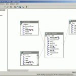
In EIS terminology, you create a model first, then a metaoutline.  A model is something you create in order to link together your SQL tables and tell EIS how they relate to each other.  At the center of this model you will have a Fact Table.  You can sort of think of the Fact Table as being similar in nature to the type of data that you would load to your Essbase cube with a normal load rule.  For example, if the rows in your data file had fields for the scenario, year, time period, location, department, measure, then a dollar amount or other figure, you can think of this as your fact table.  In this case, think of the different time periods for a moment.  In a typical periods/quarters/year setup, your text file would just have an 01 for period 01, an 02 for period 02, and so on.  Generally the source data wouldn’t make any sort of mention of the quarters, for example,  but EIS needs to know about this.  On the model, you would link the Period on the fact table to another table in your relational database that shows how to build the Time dimension based on that data.

The metaoutline has to be created after the model, because it is highly dependant on the way the model is setup.  In fact, when you create the metaoutline, you tell EIS which model to base it off of.  As the seasoned EIS veterans know about models and metaoutlines, once you commit to something in the model, you are basically married to it.  You can’t go around gutting the model too much unless you first make changes to your metaoutline(s).

If you’ve setup the model in a sane manner, you can then use the dimensions/tables you defined sort of as Lego blocks in your metaoutline, you can mix and match different dimensions and come up with a working outline.  You can even create arbitrary members in dimensions or completely new dimensions, if that’s what you need for that particular outline.  Try your best to keep it in the model though — it’ll usually pay off in the long run.

With the metaoutline properly defined, you can then load the members to a cube.  This is a straightforward process (assuming everything is setup correctly) where EIS will take your metaoutline, which is in turn based off your model, which is in turn based off your relational (SQL) data, and build a completely fresh outline for you.  Of course, this process can be automated (as with just about everything else).  If you’ve built everything correctly you can also load data through EIS too, although in practice I tend to find myself leaving that to an automation system, but it’s always good to know that your models are built properly.

The barriers to entry for setting up EIS can be daunting if you aren’t already using it.  You have to install it on a server, setup a SQL database for the metadata catalog, have some source data in SQL that you want to use to build/load outlines (which may require you to brush up on your SQL skills if you’re a bit rusty), and figure out how the tool works.  As always, learning from examples and experimenting on your own are very good ways to go — so if you can get the EIS demo app installed you should be able to see how things are put together.  The payoff though, for using EIS, can be immense.  You don’t have to mess around with all those dimension build load rules, you can spin up new outlines in a jiffy (without necessarily reinventing the wheel everytime), and girls think it’s pretty cool (and for all you female cube geeks out there, I’m sure the guys will be impressed too).

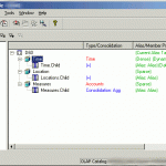
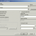
If you’re still curious about EIS (and who wouldn’t be?), feel free to drop me a line.  Also, if you’d like to see more articles about EIS, let me know and I get dig into some of the more complex stuff.  The screenshots below show some EIS screens — a model, a metaoutline, and building an outline from a metaoutline.   See in the model how the fact table is in the middle, with some other dimensions attached to it.  I blurred out some server information, but it doesn’t affect the purpose of the screenshot.

Automated EIS outline builds

Here’s a little quickie that I thought of and put in the other day. If you use the “export script” feature in EIS so that you can use that in conjunction with EIS in order to script your outline builds, you get a script that is specific to a particular server. I like to keep my test machine automation totally synced up with my production machine automation, but if I needed different scripts for different servers, then I would have to have a different automation file. Well, here’s what I did:

Name the outline build script with thte name of the server in it. I have my server name already set in an environment variable (it’s used all over the place for various automation and logging things). So if the .cbs was normally foo.cbs, and the name of the machine (prod) is bar01, and the test machine is bar02, and I reference the outline build command as foo_%SERVERNAME%.cbs, then whichever machine the script runs on, it’ll grab the right script. Kind of a small thing but I like it!

Normalize a fact table for a better EIS model

Generally I don’t load data through EIS because quite honestly, I fudged some of the EIS models when I first made them and now I’m pretty much married to them.  They are perfect for loading the outlines, but not data.  Earlier this week I was playing around with one of my newer models, trying to keep it ‘clean’ as it were, and after playing around with it, I got it set just right so the default SQL (quite a gnarly little query, really), much to my amazement, loaded exactly the data it needs from the fact table.  The one major thing I have had to tweak is the format of the fact table.  Upstream stores 3 facts in the table: for each period/location/account we store the value for the current year, prior year, and the budget value.  What I do is kind of normalize the data with a SQL script that takes all that data and puts it into a different table that has a year (YR) field and a scenario type.  This way in the EIS model, I can link this modified fact table cleanly to TIME, YEARS, SCENARIO, LOCATION, and possibly DEPARTMENTS.  It works quite nice!

Making order out of chaos with Essbase Integration Server – part 2

Last time I gave sort of a high-level look at pounding the rigid financial page definitions from the corporate overlords upstream folks, and generating the outlines based on this information. So now I have some nice fresh outlines, but I don’t have any processes for data just yet. I have a couple of issues I need to address:

  1. History is going to be restated each period so I need to go out and fetch all new data each period
  2. I need to load all of the data as fast as I can
  3. I want the data load process that runs each period to be as robust as possible.

Well, let’s start with the basics. The data I want is upstream in a DB2 server. One way to go would be to talk to the ETL group and see if they can drop off files for me each period. This isn’t really a bad option because they already deliver some pretty similar information in a similar fashion. But I don’t really feel like doing all the paperwork and cutting through the red tape right now. Since I already have a working ODBC connection, I’m just going to use this. I know, I know, ODBC is gross. I can’t really use JDBC at the moment because this particular DB2 server is z/OS and you apparently need a special .jar file to get JDBC connections to work (some kind of licensing issue). My emails to the DB2 folks about this have apparently been routed to /dev/null, and I can’t just go to the IBM download site and grab it. So that’s out for now. So let’s go with ODBC.

I determined earlier that the raw data for each period is just south of 200 megabytes. That adds up to a few gigs when you take in to account all the periods I want to look at. During the night, when network activity is relatively quiet, I can pull this down in about 20 minutes for a single period. For some reason I think this should be faster (a lot faster), but the speed seems constant regardless if I use JDBC or ODBC, so at the moment it seems like more of a network thing which I can’t change (I’m pretty sure that there is fairly extensive packet shaping going on… it’d be nice if I could have this port loosened up a bit). Maybe that’s just as fast as the DB (or my user ID on the DB) is allowed to go at. In any case, it’s tolerable, because I basically have the entire period (or one week, at the least) to pull down the history. The server has a tendency to kill my connections though, so I can’t get it all at once. I wouldn’t really prefer that option anyway, since I’m just throwing this into a text file, so I’ve decided that I would like one period per text file.

I wrote a small Python script that will read a configuration file, take some command-line parameters, and go grab all the data I want and put it into the folder I want with a particular naming convention (one period of data per file). It’s pretty nice. Source is available if anyone wants it (it’s a few pages long — nothing fancy). I used pyodbc to connect against the already setup DB2 ODBC connection. This same Python script is also flexible enough so that I can use it to pull down a single period of data — this will come in handy for scripting the period load process.

Each row of data consists of a division, location number, year, period, account, and amount. Recall that there are four different cubes in this instance that are modeled after different financial pages. The thing with this approach is that an account that is on one page may also be on another page. And based on just the account number, I don’t have a way to determine which pages the account belong to. So loading this data straight to the cubes with a load rule is out. And yes, I know that you can load data with EIS, but in this case I prefer to script the process in MaxL. Another thing about the databases is that they split out different departments in them, so I will need a way to associate the account to a department. This means that I will be loading the data files to my SQL Server database and massaging it a little bit. The massaging will be fairly minimal, because I have setup a view for each database that will do a LEFT JOIN of the ‘raw’ data to a table that associates accounts to departments to pages. I could do the JOIN in the load rule itself but that seems a bit messy, and since there are only four databases, this seems sensible.

Keeping in mind that my goal here is to be able to load all four cubes as fast as I possibly can, my process that runs at the close of each period looks something like this:

  1. Pull down current period of data
  2. Load data to SQL server
  3. Process Cube 1
  4. Process Cube 2
  5. Process Cube 3
  6. Process Cube 4

I’m using the word Process here rather than Load because these as ASO cubes, part of the process will be to design the aggregations on them that will make queries nice and snappy. The process that needs to run sometime during closing week and can be done ahead of time looks something like this:

  1. Pull down all of the historical data
  2. Load all of this data to SQL server
  3. Pull down the latest cross-reference/locations data
  4. Update outlines in staging cubes
  5. Load current data to staging cubes for validation (so we don’t get caught by any surprises if the cross-reference changed in some kind of wacky way).

What are the staging cubes? They are duplicates of the four databases but suffixed with an underscore. My original strategy with regard to these cubes was to load them, agg them, and then copy them on top of the other cubes so that the period load process would not result in any downtime for the ‘real’ cubes, but along the way I have discovered that I can load these babies up fast and in a scripted fashion, and that I am better off just loading direct. Also, the MaxL process ‘create or replace…’ seems to really shake the server to its knees and doesn’t have the best performance. Right now I keep the “_” cubes around for testing purposes. This hasn’t resulted in a duplicate of scripting functionality though, I just have a text file with a list of app/db names that I pass to a batch file, so I can choose which cubes to work with just by feeding a different configuration file.

The load process for each cube, then, simply clears the data, loads it (directly from SQL Server), and aggs it.  I have tweaked the essbase.cfg to try and use 16 threads (the servers are quad-proc Xeons) and the speed seems much improved even from specifying 8, and definitely faster than none at all.  The connection between the SQL server and the Essbase server is all gigabit with a theoretical 125 MB per second of throughput, although in actuality the throughput is much less than this.  Altogether, just under a billion or so facts are loaded up and calculated (aggregrated) in about 40 minutes.

It’s not necessary right now, but a few areas that I could shave time off of would be to pre-stage the historical data that is in SQL to a text file on the Essbase server itself, then load this to a buffer, then load the new data.  I could also use a different load rule that doesn’t need to prefix the various members with our naming convention (Lo. for a location, etc), so that the load rule has to do less ‘thinking,’ but again, this hasn’t been necessary.  If it were, I’d be very curious what kind of performance we could squeak out by attaching three more drives to the storage array and setting up a partition on them so that it was separate than the drives with the Essbase data, then the disk wouldn’t be needing to read and write from the disks at the same time.

Making order out of chaos with Essbase Integration Server – part 1

Essbase has been a great addition to the decision-support toolbox in our enterprise due to the fact that the financial pages are produced via a “home-cooked” solution. It’s actually quite impressive, although in some ways I would say that it is limited due to it’s rather rigid structure. Our world consists of seven-digit accounts for everything. You can glean a little bit about what the account is based on what digits are where, although don’t count on it. Accounts are then associated with lines (NET SALES, GROSS PROFIT, RENT, EBITDA, etc), and the lines make up the “physical pages.” The lines are numbered 00 through 99 and they quite literally correspond to a position on a piece of paper. 00 is the first line, followed by 01, then all the way to the next page with 99 on it. It’s not necessary to use all the lines, in fact, many of them are blank. Accounts are then directed towards lines. They are not “nested” in a true hierarchy — an account is simply directed multiple times. For example, sales for a particular department are directed to the NET SALES line, but since it also affects GROSS PROFIT, that particular account is also directed to the GROSS PROFIT line. This is all maintained in the Cross Reference, which is the master list of all report types and account groups (basically just different accounting systems for different business segments), the account, the line it rolls to, a description of the account, and a description of the line.

The trick, then, is how do we make this useful in Essbase? It is our goal to mirror the financials, and provide a window into them that previously did not exist, but essentially our Measures dimension is a fairly fast moving target. It can (and is) changed at any time, and we have anywhere from 5,000 to 80,000 accounts that affect a single financial page (the decision to model separate cubes after particular groups of financial pages was made long ago to make the cubes more manageable and to make more sense to the end-users). We also need to be able to load the data for a new financial period right after it closes. So altogether, here’s what we know:

  1. The Measures dimension has tens of thousands of members, and they change every periods (additions and deletions).
  2. The Measures dimension is a ragged hierarchy based on the way the accounts roll up on the financial page itself.
  3. The Location dimension changes each period, as well as the Attribute dimensions that are associated with the Location dimension.
  4. The raw data for a single period of data is about 200 megabytes (a straight, tab-delimited pull from DB2)
  5. In this particular case, there will be four cubes modeled after four different groups of financial pages. This means that data will be loaded four times.
  6. Data will be final (the books closed for a particular period) at 4AM Eastern time. All databases must be loaded and ready by 7AM.

Although using BSO isn’t automatically ruled out in this scenario, it was definitely not a favored option. The databases in this scenario will easily be tens of gigabytes each. These databases essentially already exist at just one division and a single period start to finish is many hours. ASO was the obvious choice. ASO has a few quirks, probably the most notable is that when you touch the outline, you lose all the data. So this means that we are going to load all of the data, for all periods and all years, every period. This isn’t really a bad thing though — due to history restates occurring for possibly any location and any measures, it is basically necessary to reload all historical data each period anyway.

Well, let’s tackle the issue of the outlines first and worry about the data second. Essbase Integration Server (EIS) was an obvious choice for this. The cross-reference and list of locations are both stored on the WAN and in a DB2 system. The Essbase and SQL Server boxes are in a different state, but all on the same LAN as each other. The format of the cross-reference data — that is, that way that everyone else looks at it besides the Essbase folks — isn’t really usable for us in its present state. We’re going to need to massage it a little bit. In this case, because I need the data on my on SQL box, and I want it on the same LAN as Essbase (so I can test faster, among other things), I will setup a quick DTS job to pull the data down for me.

The Merant DB2 drivers are garbage, so I found some IBM DB2 ODBC drivers to setup on the SQL box, then hook up the DTS job. This is SQL Server 2000 (ugh), otherwise I would have used whatever they call it now (SSIS?). It’s about 3 million rows altogether and takes a little while to pull down. I can automate this in the future, but for now I am content to just refresh it by hand once a period. Now I have my vey own cross-reference, yay! I setup some views on it for convenience (to split up some fields for me), and indexed on the physical page to make some of my queries a bit snappier. I did the same thing for the list of locations (all five-thousand or so) that I’m also pulling down in a DTS job.

The Measures dimension is quite ragged, so I chose the Parent / Child method of building things in EIS. My final table that I will use as the source data for EIS generally is of the form Parent, Child, Alias, Agg, UDA, Formula, SolveOrder, OrderWeight, and DataStorage. This works out pretty well for me and gives me everything I need for EIS. I don’t generally need more alias tables, if I did I would probably just bust out another table and do a physical join on some ID. With some fairly simple Transact-SQL, I have written a script that generates the dataI want (all the children and their parents). I used some temporary tables, some REPLACEing, and a few other tricks. Of special note, due to the sign on accounts that are in GROSS PROFIT, I have tagged these accounts with a UDA (‘GP’) so that I can do sign flips on it when I go to load that particular cube.

Speaking of ragged hierarchies, Location is ragged too so I setup some T-SQL to translate that from a flat structure (store — zones — division) into Parent/Child as well.  I took care in EIS to setup the model carefully so I could use it effectively for all four of the cubes.  Whip up some build scripts so that the outline updates can be scripted, and we’re golden.  The outline update process only takes about a minute for each cube — keep in mind that the data is dumped from the get-go, making things substantially faster.

Next time: data load strategies with an emphasis on loading as fast as we can.