Dodeca Dynamic Grouping with Relational Data

I am very pleased today to write about an incredibly awesome Dodeca capability: dynamically built groups based on relational data. This capability is interesting and useful for a variety of reasons. Using Dodeca’s spreadsheet/data/magic build paradigm, we can organize plain relational data into beautifully formatted, insightful, and dynamic views. Just to forecast where I’m headed with this, what we’re going to do is transform this plain relational data:

Some raw forecast related data

Some raw forecast related data

Into this dynamic, grouped, and formatted view:

Dodeca dynamic grouping opened up in Excel

Dodeca dynamic grouping opened up in Excel

And further, we’re going to do it without writing a single line of code (save for the simple SQL Select statement). This post will assume that you’re up and running already with Dodeca’s SQL Passthrough DataSets, which I have written about before, so head over for a refresher if you need it. Also, I’ll be recycling a simple SQL table with forecast data by employee that I also used in an earlier Dodeca relational database input article, so you can read that if you want to know more about the data in play and how it relates to Sample/Basic. Continue Reading…

Data Input with Dodeca, part 5 – Relational Database input

I have been really, really looking forward to writing this continuation in the Dodeca Data Input series, for a couple of reasons. For one, it’s a genuinely useful feature that Dodeca implements very well. But secondly, and perhaps more important, the ability to get and store this data from users is just an absolutely missing piece of functionality in the traditional Hyperion toolbox. So this is going to be a bit of a long article but will cover how relational data input in Dodeca works and why it’s so important.

As a quick recap, up to this point I’ve covered basic Essbase data input, cell/variance commentary, going under the hood to look at the audit log tables, and focused calc scripts that run after Essbase input. To this we will now add SQL/relational data input. To put it in context, relational database input is one of the tentpole Dodeca features, and stands next to other heavy hitter features such as Essbase input, comments, drill-through, and cascading reports. Now, all of the individual features of Dodeca are useful and interesting. And yet, I see relational data input as a feature that almost singlehandedly makes Dodeca greater than the sum of its parts.

Relational Data as Part of the Hyperion Toolbox

Before jumping in to the technical implementation of relational data input in Dodeca, I want to wax philosophical a bit on how important I think this feature is. It has the power to be a game changer for a lot of organizations.

My own experience with Hyperion/Essbase is from all angles: as a full-time Hyperion developer for multiple companies, as a consultant with multiple companies, working on dozens projects, and as an independent software vendor with a Hyperion product. Further, my computer science degree minor was in relational database algebra (yes, I’m a nerd). I wrote the innovative Drillbridge software that bridges the gap between Smart View, Planning, and Financial Reporting and relational data. I created an absolutely free version of the Drillbridge software that is fully functional and is downloaded daily and regularly put into production with zero assistance from myself.

So to say that relational data is near and dear or otherwise useful to me is an understatement. As with Dodeca’s robust and battle-tested middle tier component (the secret sauce/glue between the Dodeca client application and all Essbase/relational database servers), Drillbridge is written in 100% Java and contains a web interface for managing its configuration.

All that background is basically my long-winded way of saying that I’ve worked with Hyperion a lot, and if anyone should be qualified to find a way to get user input into a relational database, it’s the guy that programs in Java, writes CDFs for fun, and has created systems that literally take input from a user and put it into a relational database.

And yet, even with all of this experience, getting relational data from Hyperion users has traditionally been this absolute missing link. The situation with pure Essbase data has been a little better: you had lock and send or submit data with the classic add-in/Smart View. Of course, lock and send is not without it’s issues. It’s more of a power user thing, although as I’ve explored in the past, Dodeca can quite nicely provide some structure to the Essbase input process that makes things much more user friendly.

Essbase Relational Data Input Anti-Patterns

I seem to harp on this notion of anti-patterns a bit. An anti-pattern occurs when something is ostensibly designed incorrectly. This happens a lot in the Hyperion consulting world, for instance. A client might be having an issue with their system or performance, and they come to a consultant looking for assistance on that one particular symptom. Unfortunately, all too often, the performance or technical problem is essentially predicated upon a series of unfortunate business, technical, and design decisions (usually ones that can’t be easily/cheaply rectified). Or the company has otherwise accumulated a lot of technical debt – where band-aids have been put on a system in order to keep it hobbling along, without addressing the underlying design problem.

Armed with only Smart View or the classic add-in, but needing to get relational input from users, an intrepid (or masochistic) Hyperion developer might choose a few different routes to try and satisfy this, all of which are less than ideal for various reasons;

  • Dummy members/dimensionality for pseudo relational input
  • Text measures
  • Enter supporting details/data to Excel spreadsheet, and email to admin or store on share folder/drive
  • Custom VBA program/functionality to upload supplemental detail
  • Custom software/web service for user to input data

All of these approaches have issues. Adding dummy members or attributes to a cube is less than ideal and “pollutes” the cube. Some additional functionality might be needed to pull that data out of the cube and marshall into a relational database. Sending emails and saving spreadsheets off to the local share drive is a disaster waiting to happen. I’ve railed on VBA solutions before. They are a mixed bag. Speaking as a consultant, they all too often turn into spaghetti code maintenance nightmares, fraught with glitches, security issues, and more. Lastly, a custom web service or software package might fit the bill, but it takes time and money.

Dodeca Does It (#dodecadoesit)

Let’s explore some what-ifs:

  • What if users could input data using the same interface they are using for reporting and analysis
  • What if we didn’t need to make a single change to our cube dimensionality and cube get relational input from the user
  • What if it didn’t require any custom programming, save for the SQL statements themselves
  • What if we could work with almost any major relational database technology on the planet
  • What if this functionality was a first-class citizen in our software and worked out of the box?
  • What if we could format the data to our heart’s content using a spreadsheet model that we already work with day in and day out?

Here’s the thing: Essbase ostensibly started its life not really caring at all about SQL/relational data. As has been wistfully recalled time and again, Essbase was the secret weapon sitting under your desk. The classic Excel add-in could magically slice and dice data. Over the years, Essbase – and users, whether they realized it or not – grew to have an increasingly important relationship with relational data.

Even the most experienced of Hyperion developers is often at a loss when it comes to providing their users a cohesive solution that can seamlessly work with relational and multi-dimensional data (or OLTP/OLAP if you prefer). And yet, this is a bread and butter feature of Dodeca. It feels almost hyperbolic to say, but I just can’t stress this enough.

Okay, enough with the abstract and architectural. Now let’s move on an actual implementation inside of Dodeca that writes back to a SQL table of our choosing.

Implementing Relational Data Input With Dodeca

For the remainder of this exercise, we’re going to work with a table called EMPLOYEES. It’s a very simple table that contains a employee ID, first name, last name, and a comment about a given employee. The employee ID must be unique (it’s the primary key). The other fields are just made of text. Thy MySQL table definition would look like this:

CREATE TABLE `EMPLOYEES` (
    `EMPLOYEE_ID` int(11) NOT NULL AUTO_INCREMENT,
    `FIRST_NAME` varchar(25) NOT NULL,
    `LAST_NAME` varchar(25) NOT NULL,
    `COMMENTS` varchar(255) DEFAULT NULL,
    PRIMARY KEY (`EMPLOYEE_ID`)
)

Also note that the EMPLOYEE_ID field is an AUTO_INCREMENT value. This is MySQL’s equivalent of a SQL Server identity column, or using a sequence in an Oracle table to generate the next unique value. Essentially what this means is that the database engine itself will take care of creating new values for us, so we don’t (in fact, we don’t want to) insert them manually or ourselves. However, we will be interested in the value that the database engine assigns to the rows we insert. You’ll see later how this is accomplished.

I went ahead and put in a couple of rows using a generic database tool and built a very simple Dodeca view that pulls back the data. Here’s a preview of that:

A basic Dodeca view with relational data

A basic Dodeca view with relational data

One of the blog posts leading up to this one was a quick crash course in how to put relational data into a Dodeca view, so if you’re fuzzy on that, then I suggest you take a look at that. But in a nutshell, here’s what is going on with respect to the template:

Basic template for relational view

Basic template for relational view

Things to note:

  • The range that will be populated with data from the relational query is named EmployeeComments and contains four columns (one for each column we retrieve with the query)
  • I turned on the option to return the headers from the query; those will be populated into the first row of the range. This can be turned off and custom headers can be supplied, but in this case I want to just use them
  • I’ve applied some light formatting to spruce things up a bit: row 2 (the first row of the range) is grey with white text, and I added a spacer row/column to offset the table a little bit. I’m going to set the options on this view to not show row/column headers or the different tabs (again, just settings that I can easily update)

Note the Grid Properties settings that I’ve updated for the view, in order to enhance the visual appearance of the rendered view for the user. In particular, I’ve turned off grid lines (GridLinesVisible = False), headers for the cells won’t be displayed (RowAndColumnHeadersVisible = False), and tab names won’t be displayed (TabsVisible = False).

Updated Grid Properties for relational Dodeca view

Updated Grid Properties for relational Dodeca view

Next we need to use the DataTable Range Editor to tell Dodeca a little about how the SQL Passthrough DataSet we defined earlier is rendered into the named range on our sheet. In the previous post looking at this functionality, we got to leave many of the configuration values as their defaults. This time we need to set a few more things in order to allow user input in addition to viewing the data.

DataTable Range Editor associated with the SQL passthrough dataset on our view

DataTable Range Editor associated with the SQL passthrough dataset on our view

Of particular note in this editor:

  • The DataSheetRangeName is set to the named range from our Excel template (EmployeeComments)
  • The SetDataFlags configuration value includes a value of InsertCells (note that the SetDataFlags parameter can accept multiple values; in this case we are setting just one of of them).

Now let’s cut over to the Query Editor associated with our SQL Passthrough DataSet and take a look at the configuration there:

Query Editor editing the SQL passthrough dataset for employees

Query Editor editing the SQL passthrough dataset for employees

Now, it looks like there is a lot going on here but it’s not too bad. Let’s walk through all of the things that are set in this query. Also remember that the this query configuration is associated with the SQL Passthrough DataSet itself. In other worse, this is the type of logic that we only need to configure in one place and we can then reuse across multiple views if we want (as opposed to having to reinvent this configuration/logic for each individual view).

The important aspects of this query configuration are the SQLConnectionID, DataTableInfo/Columns, and the values in the SQL configuration (InsertSQL, SelectSQL, and UpdateSQL):

  • SQLConnectionID: this is the simplest item to configure. We simply use a dropdown box to choose from our list of SQL connections that have been mapped in previously. We set this regardless of writing data back to SQL or not (we need to set it even if we’re just reading data from SQL, obviously)
  • DataTableInfo/Columns: often these don’t even need to be set because Dodeca can figure them out dynamically. It depends on the JDBC driver in play. I went ahead and created mappings for the columns just to make sure that there would be no issues with reading the column names and types out. The editor for creating these is straightforward and is purely just a literal column name and a column type (int, varchar, datetime, etc.). Additionally, I also explicitly told Dodeca what the primary key for the table is (EMPLOYEE_ID).
  • The SelectSQL configuration is the exact same as before (when we we’re just reading data out of SQL), so nothing new to see there. What’s new is the configuration for the InsertSQL statement.

Let’s take a closer look at the exact configuration of the InsertSQL parameter, as it’s possibly one of the more interesting nuances in this whole configuration. The InsertSQL setting is ostensibly just the parameterized SQL code to insert a new row into the table, however, in this case we actually have two statements (one per line in the following screenshot):

The InsertSQL value for the employees query on the employee SQL passthrough dataset

The InsertSQL value for the employees query on the employee SQL passthrough dataset

The first statement is the parameterized INSERT. The full statement is INSERT INTO EMPLOYEES (FIRST_NAME, LAST_NAME, COMMENTS) VALUES (@FIRST_NAME, @LAST_NAME, @COMMENTS). I want to draw your attention to the fact that I am explicitly not mentioning the primary key (EMPLOYEE_ID) here. Recall that this is the primary key but also an AUTO_INCREMENT (similar to IDENTITY/sequence in SQL Server/Oracle respectively). I’m basically telling the relational database engine “Hey, I’m going to explicitly give you these three things, but you’re smart enough to figure out how to automatically generate the key for me, so please do that.”

Inside of the VALUES section of our insert statement, you’ll see that we have tokens starting with an @ symbol: @FIRST_NAME, @LAST_NAME, and @COMMENTS. When Dodeca goes to do the insert, it’ll dynamically place the values from the row into these placeholders and then execute the query. So to be clear, these aren’t part of the native SQL syntax. For instance, if I am inserting my own name and comments into the row and then have Dodeca save it, the resulting SQL statement that Dodeca generates and then hands off to the database for processing might look like this:

INSERT INTO EMPLOYEES (FIRST_NAME, LAST_NAME, COMMENTS) VALUES ('Jason', 'Jones', 'Awesome employee')

The next statement, and one that’s incredibly useful to our user experience, is the “post insert SQL” command. The code for this post insert command in this case and for this technology is the following:

SELECT EMPLOYEE_ID, FIRST_NAME, LAST_NAME, COMMENTS FROM EMPLOYEES WHERE EMPLOYEE_ID = LAST_INSERT_ID()

Take special note that there is a semi-colon at the end of the first line that is separating the insert command from our special post-insert command. With respect to the post insert command, there are no special tokens in it, but it is specific to MySQL in this case. In particular, the LAST_INSERT_ID() function is a special function that returns the generated ID for the row that was just inserted in the previous statement. Effectively what I’m telling Dodeca is this: “After you insert the first name, last name, and comments to the relational database table, a primary key will have been generated. Here’s how you can use that generated primary key to fetch all of the details for that row, so that you can populate the key on my spreadsheet.”

Let’s go ahead and take a look at how this looks on the spreadsheet and the user experience. With my view all configured, let’s run it and take a look:

The Insert Row button on the toolbar is enabled when the cursor is inside a value input range

The Insert Row button on the toolbar is enabled when the cursor is inside a value input range

I apparently have two employees in this absolutely fictitious company. As you can see, there’s myself, and then there’s Cameron Lackpour. Apparently Cameron likes CALC ALL;. He also really likes load rules, low block density, and inputting to upper level members. But that’s neither here nor there. Anyway.

You can see in the spreadsheet that my cursor is located within the data table somewhere. Because of this, the Insert Row button is active. Take a look at the button toolbar and about in the middle you can see there are some table row-related icons. The Insert Row button is the third button to the left of the “100%” zoom indicator. I simply click on that to insert a new row to the table:

Finished entering data to be sent to the SQL database, but not saved yet

Finished entering data to be sent to the SQL database, but not saved yet

As you can see, I’ve added a new employee and comment. It’s Tim Tow and he apparently knows a thing or two about Excel. The row has not been sent to the database just yet. I will use the Save button on the toolbar (directly to the left of the 100% zoom indicator) to save this row.

Remember, behind the scenes, Dodeca knows that the value of FIRST_NAME is 'Tim', LAST_NAME is 'Tow', and COMMENTS is 'Excel ninja'. So it takes care of all of the ugly work of turning those raw inputs into a valid SQL query, using the statement we provided, talking to the relational database, getting the result back, and in this case, immediately executing the post-insert SQL statement. Immediately after pressing Save, our sheet looks like this:

New row saved and primary key value is automatically updated

New row saved and primary key value is automatically updated

It’s basically the same, save for one thing: the newly generated primary key for the row we entered has been pulled back (along with the rest of the new row) and dynamically updated into the view – with no refresh needed.

Conclusion

This was a very long article that covered aspects of architecture, Essbase anti-patterns, Cameron Lackpour’s love of load rules, and a real example of using Dodeca to write back to a relational table. There are many more nuances to the SQL data editing/updating that I’ll explore in future posts, such as updating existing rows, deleting rows, data grouping and more. But I wanted to give a practical crash course on the basics of this incredibly useful feature. Relational data input is an incredibly useful and important ability to have in so many organizations, and yet when the need for this type of capability arises on the Hyperion side of things in many organizations, all too often there isn’t a compelling, cohesive, and maintainable way to achieve it – but Dodeca does it.

Data Input with Dodeca, part 3 – Data Audit Log

Welcome back to the Data Input with Dodeca blog series! We’ve already covered a good bit of ground already. To start things off, we looked at basic data input to an Essbase cube using Dodeca, then we looked at how to let users provide commentary on their Essbase data input. These are both incredibly useful features, but perhaps more importantly, form the cornerstone of many typical Dodeca applications.

Today I want to dive under the hood a bit and look at the Dodeca data audit log. Whenever data is input by a user, it’s logged. This one of the important legs of the data input stool (in addition to comments) and greatly complements data comments. Whereas data cell commentary might be thought of as being useful in a business context, the data audit log is probably more useful in an IT and SOX context. The rest of this article is going to focus on the technical details of the data audit log, while subsequent posts in this series will take a look at putting a friendlier face on it.

The Dodeca data audit log is comprised of three main tables that reside in the Dodeca repository itself. So there’s no additional setup to worry about – these tables exist out of the box.

Data Audit Log Tables

These tables are DATA_AUDIT_LOG, DATA_AUDIT_LOG_ITEMS, and DATA_AUDIT_LOG_DATAPOINTS.

DATA_AUDIT_LOG

The DATA_AUDIT_LOG table contains records of all the overall data input activities. A single data input operation may affect multiple cells of data; all of the affected cells of that are modified in a particular user action are grouped together. This table contains the audit log number (an integer primary key), the Dodeca tenant, the Essbase server/application/cube, the user, and the date the data was modified.

DATA_AUDIT_LOG_ITEMS

There are one or more audit log items associated to a single audit log. In other words, if the data audit log contains a list of transactions, then the audit log items are the list of cells (however many that my be) that were edited in that transaction. This table contains a unique ID (primary key), an association (foreign key) to the audit log table, the old value of the cell, and the new value of the cell. Note that it doesn’t not contain the members from the dimensions (that’s coming up next).

DATA_AUDIT_LOG_DATAPOINTS

The DATA_AUDIT_LOG_DATAPOINTS table contains the member names of cells that were modified. For example, consider our friend Sample/Basic. A sample intersection that was modified might be Sales, Budget, Jan, 100-10 (Cola), Washington. Each one of these would be represented as a single row in the data points table.

All Together, Now

The fully normalized format for storing modified data points tells us absolutely everything we want and need to know about data that is modified. We know the who (user), what (old value, new value), where (Dodeca app, Essbase app/cube, intersection), and when (created time). As for the why – that’s more of a commentary thing.

Given that we have all of this information, and given that it’s stored in a nice normalized form in a standard SQL database, we can query it and view/answer all manner of questions about the data. This opens up some very cool possibilities:

  • Query the database directly to see what changed, if anything
  • Setup an ETL process (ODI!) to provide a regular report of modified data (extra useful during the forecast cycle)
  • Build a view in Dodeca itself that will allow us to query the modified data using standard Dodeca selectors (coming to a future blog post)

For now, let’s take a look at some example queries to get an idea of what we’re working with. The Dodeca repository that I’m working with the moment will be a MySQL schema. MySQL is one of the many relational database technologies that Dodeca works with. The most common ones are Oracle, Microsoft SQL Server, and DB2. But I like my Dodeca servers on a nice compact Linux server, and MySQL fits the bill quite nicely. I’ve tried to write the SQL in the most generic way possible so that if you want to borrow it for your own repository it shouldn’t need any major modifications.

To start things off, let’s say we just want a list of all of the modified data, by user, by modification time, with all data points (this could potentially bring back a lot of data in a large repository, by the way):

SELECT
    AUDITLOG.SERVER,
    AUDITLOG.APPLICATION,
    AUDITLOG.CUBE,
    AUDITLOG.USER_ID,
    AUDITLOG.CREATED_DATE,
    DATAPOINTS.MEMBER,
    DATAPOINTS.ALIAS,
    IFNULL(ITEMS.OLD_VALUE, '#Missing') AS OLD_VALUE,
    ITEMS.NEW_VALUE
FROM
    DATA_AUDIT_LOG_DATAPOINTS DATAPOINTS,
    DATA_AUDIT_LOG_ITEMS ITEMS,
    DATA_AUDIT_LOG AUDITLOG
WHERE
    DATAPOINTS.AUDIT_LOG_ITEM_NUMBER = ITEMS.AUDIT_LOG_ITEM_NUMBER AND
    ITEMS.AUDIT_LOG_RECORD_NUMBER = AUDITLOG.AUDIT_LOG_RECORD_NUMBER
ORDER BY
    AUDITLOG.CREATED_DATE;

Note a couple of things:

  1. Data is sorted by date, oldest to newest
  2. There’s an inner join between the three tables, you must make sure that all tables are joined together
  3. Data that was or became #Missing will be null in the table. For niceness I have used an IFNULL here to convert it to #Missing. Oracle’s equivalent is NVL. SQL Server uses COALESCE.
  4. This table will contain one row per dimension per modified data point (as opposed to one row per modified cell).

Okay, that’s all well and good. How about we filter things a bit and we only want to see data points that were modified in the last 30 days? Just add a simple predicate:

SELECT
    AUDITLOG.SERVER,
    AUDITLOG.APPLICATION,
    AUDITLOG.CUBE,
    AUDITLOG.USER_ID,
    AUDITLOG.CREATED_DATE,
    DATAPOINTS.MEMBER,
    DATAPOINTS.ALIAS,
    IFNULL(ITEMS.OLD_VALUE, '#Missing') AS OLD_VALUE,
    ITEMS.NEW_VALUE
FROM
    DATA_AUDIT_LOG_DATAPOINTS DATAPOINTS,
    DATA_AUDIT_LOG_ITEMS ITEMS,
    DATA_AUDIT_LOG AUDITLOG
WHERE
    DATAPOINTS.AUDIT_LOG_ITEM_NUMBER = ITEMS.AUDIT_LOG_ITEM_NUMBER AND
    ITEMS.AUDIT_LOG_RECORD_NUMBER = AUDITLOG.AUDIT_LOG_RECORD_NUMBER AND
    AUDITLOG.CREATED_DATE BETWEEN CURDATE() - INTERVAL 30 DAY AND CURDATE()
ORDER BY
    AUDITLOG.CREATED_DATE;

Please note that SQL languages differ wildly on their date math. I think the Oracle analogue here is relatively similar but SQL Server’s is a fair bit different.

Okay, how about if we’re only interested in a particular product being modified? Let’s filter on the member name/alias:

SELECT
    AUDITLOG.SERVER,
    AUDITLOG.APPLICATION,
    AUDITLOG.CUBE,
    AUDITLOG.USER_ID,
    AUDITLOG.CREATED_DATE,
    DATAPOINTS.MEMBER,
    DATAPOINTS.ALIAS,
    IFNULL(ITEMS.OLD_VALUE, '#Missing') AS OLD_VALUE,
    ITEMS.NEW_VALUE
FROM
    DATA_AUDIT_LOG_DATAPOINTS DATAPOINTS,
    DATA_AUDIT_LOG_ITEMS ITEMS,
    DATA_AUDIT_LOG AUDITLOG
WHERE
    DATAPOINTS.AUDIT_LOG_ITEM_NUMBER = ITEMS.AUDIT_LOG_ITEM_NUMBER AND
    ITEMS.AUDIT_LOG_RECORD_NUMBER = AUDITLOG.AUDIT_LOG_RECORD_NUMBER AND
    AUDITLOG.CREATED_DATE BETWEEN CURDATE() - INTERVAL 30 DAY AND CURDATE() AND
    (MEMBER IN ('Cola') OR ALIAS IN ('Cola'))
ORDER BY
    AUDITLOG.CREATED_DATE;

Just to hit this home a bit, here’s a screenshot of the data that comes back for my local server, using one of my favorite SQL tools, RazorSQL:

Sample query on the Dodeca repository data audit log tables

Sample query on the Dodeca repository data audit log tables

As I mentioned earlier, one of the really interesting things we can do with Dodeca is to built a view in Dodeca itself that will allow us to easily filter and see what’s going on with the data, by tapping into Dodeca’s own repository. But in the meantime I hope you found this article helpful and saw some of the possibilities that are afforded to you. Invariably when I discuss this tool with people, there is a conversational progression of yes answers that lead to data audit logging:

Does it handle data input?

Does it handle data input comments?

Is there an audit log showing me which data was modified so that I can make my IT Risk/Compliance/SOX department happy, please say yes, please say yes?

Yes!

Vess Updates Substitution Variables

A colleague of mine is running into an issue with substitution variables and was looking for a solution that he could use to sync values up. He thought maybe Vess would be a good fit. Vess, as I have blogged about before, is a “virtual” Essbase JDBC driver. Vess maps Essbase concepts and crams them into a typical database model. For example, Vess exposes tables that model substitution variables.

In the case of server-wide substitution variables, there is a “VARS” table that has two columns: NAME and VALUE. For each application, there is another table that contains four columns: NAME, VALUE, APPLICATION, DATABASE.

As a quick aside, this might seem a little odd to have separate tables. After all, this table is notionally about the same as the Variables screen in EAS. Well, you have to kind of flip your thinking a little. Don’t think of variables as being only either server or a cube: think about in terms of what variables are applicable to a cube. In other words, if you ask Essbase what variables are applicable to the whole server, then this would be the global variables only. If you ask Essbase what variables are applicable to a cube, then it’s the cube, app, AND the server specific variables. This is one of the reasons there are multiple tables to model the variables.

Getting back on track, given that we have these tables and we can treat them just like normal SQL tables, we can do some interesting things. Let’s say we want to create or update a variable specific to an app that exists in the global scope. We can do this in one line:


INSERT INTO SAMPLE.VARS<br />
SELECT NAME, VALUE, 'Sample', 'Basic'<br />
FROM VESS_SCHEMA.VARS WHERE NAME = 'Foo';

What’s going on here? In Vess, a schema named VESS_SCHEMA is presented for server-wide things (server wide variables are in the table VARS in this schema, as shown above). The server VARS table only has columns NAME and VALUE.

Each application on the Essbase sever is modeled as its own schema. In this case, our favorite app – Sample – gets a schema named SAMPLE. This schema also contains a VARS table (containing columns NAME, VALUE, APPLICATION, and DATABASE).

Given these tables we have, it’s a simple matter of selecting the server variable with the name we want (in this case, a variable named ‘Foo’), and insert it into the variables for the Sample app.

Of course, if we wanted to for some reason, we could alter the name using normal SQL (string truncating, substrings, etc), or whatever. We can also delete variables, such as this:


DELETE FROM SAMPLE.VARS WHERE CUBE = 'Basic';

As I’ve said before, Vess continues to be an “interesting” proof of concept. As time permits I am filling out more and more functionality. At present, Vess models things like substitution variables, metadata you might see in MaxL or EAS (cube statistics, user sessions, etc), can load data to cubes, and can do certain outline related operations.

Vess is not available as a public download at this time but I have handed a few copies out to get feedback. I think Vess is just about good enough to be used in automation and other things. If you’re interested in using this in a production situation (automation or otherwise), please contact me to discuss support options.

Manually injecting rows to an ODI journal table

Earlier this year I did an absolute whirlwind crash course on ODI journalization. In that article I talked about the layout of tables that ODI uses to track changes in particular tables (for simple journalization with one table). You may recall that changed (inserted, updated, deleted) rows are tracked in this table. This is done by way of some metadata as well as the primary key of the monitored table.

Typically after your processing is done, the entries from the ODI journal table that were processed will be deleted. Occasionally, however, you may need to manually fix the ODI journal table. For me this sometimes involves “manually injecting” rows to the journal table. You could achieve this in a couple of ways. This way we can force some rows to process that otherwise wouldn’t be processed because ODI doesn’t consider them to be new or updated.

The first way is to “touch” the rows in the monitored table in some way so that the trigger installed on that table gets activated and inserts rows to the ODI journal table. You could perform some sort of dummy update on a row. This can work but isn’t always desirable.

Another technique and the one I’ll talk about in this post is to manually add rows to the journal table that contain the primary key of the row to be processed. The trick, then, is what to fill in for the other values of the columns?

Recall that the general format of a table is the subscriber name, a consumed flag, the date it went into the table, whether it’s an insert or a delete, and the primary key of the row being journalized.

As an example, assuming the journal table is called J$TEST_CODE_RESULT (for a real table of TEST_CODE_RESULT), and also assuming a primary key name of TEST_CODE_RESULT_ID (that in this case is an integer), we can add a row to the journal table like this:

INSERT INTO TEST_CODES.J$TEST_CODE_RESULT VALUES ('TEST_CODE_PROCESSING', 0, 'I', sysdate, 12345);

The first value is the JRN_SUBSCRIBER. This corresponds to the name of the subscriber setup in the ODI journalizing and is also the same as the filter you use in the interface to get rows for just your particular subscriber. Next is the JRN_CONSUMED field which we set to 0 (during processing, ODI will change this to 1 to indicate it’s working on that data), the character ‘I’ (upper case i) to indicate the row was an insert or update, the current time (this assumes an Oracle database), and finally, the ID of the row we need to inject.

You can of course also insert as many rows as you want such as by writing an INSERT that gets values from a SELECT. Every now and then if you have a lot of rows you need to reprocess you might find yourself with a table that has the IDs, and you can just insert them into this table and they’ll get picked up on the next run.


Pump data into an Essbase cube directly from a relational database with just Java and no load rule using Hyperpipe

Kind of a wordy blog title. There is plenty of more information on the Github project page.

Based on a conversation with Cameron Lackpour, I wrote a small utility that can move data from any JDBC data source to an Essbase cube. You don’t need MaxL, a load rule, ODBC, ODI, or any of that stuff.  I mean, you might want to use those things instead of this odd little one-off utility, but if you like living on the edge you can give this a try.

Hyperpipe works by piggybacking off some functionality that is already in the Essbase Java API. Craft a SQL query in a particular format and you can load up an Essbase cube without having to make a load rule or jump through too many other hoops. This could be useful in some situations. Hyperpipe is believed to work with all Essbase versions 9.3.1 or higher but has not been extensively tested. Hyperpipe is an open-source project released under the liberal Apache Software License — a business-friendly license that you can do pretty much anything you want to.

Please try it out if you’re interested and let me know if you have any questions, comments, suggestions, or issues.

Happy cubing!

A comprehensive Essbase automation optimization story, or: Shaving off every last second

I’ve been wanting to write this post for awhile.  Like, for months.  Some time ago I took an in-depth look at profiling the performance (duration-wise) of an automated system I have.  The system works great, it’s worked great, I don’t need to touch it, it just does its thing.  This is the funny thing about systems that live in organizations: some of the rather inglorious ones are doing a lot of work, and do it reliably.  Why reinvent the wheel and risk screwing things up?

Well, one reason is that you need to squeeze some more performance out of that system.  The results of my profiling efforts showed that the process was taking about an hour and a half to run.  So, considering that the processing of the data is an hour behind the source system (the source system drops off text files periodically for Essbase), and it takes an hour and a half to run, the data in the cubes is some two and a half hours behind the real world numbers in the original system.

So, first, a little background on what kind of processing we have here.  The gist of how this particular system works is that a mainframe manages all of the data, and certain events trigger updated files to get delivered to the Essbase server.  These files are delivered at predictable intervals, and automation jobs are scheduled accordingly (about an hour after the text files are scheduled to be delivered, just to be on the safe side).  The data that comes in is typical financial data — a location, a time period, a year, an account, and an amount.

Pretty simple, right?  Well, there are about twenty cubes that are financial in nature that are modeled off of this data.  The interesting thing is that these cubes represent certain areas or financial pages on the company’s chart of accounts.  Many of the pages are structurally similar, and thus grouped together.  But the pages can be wildly different from each other.  For this reason, it was decided to put them in numerous cubes and avoid senseless inter-dimensional irrelevance.  This keeps the contents of the cubes focused and performance a little better, at the expense of having to manage more cubes (users and admins alike).  But, this is just one of those art versus science trade-offs in life.

Since these cubes add a “Departments” dimension that is not present in the source data, it is necessary to massage the data a bit and come up with a department before we can load the raw financial data to a sub-cube.  Furthermore, not all the cubes take the same accounts so we need some way to sort that out as well.  Therefore, one of the cubes in this process is a “staging” database where all of the data is loaded in, then report scripts are run against certain cross sections of the data, which kick out smaller data files (with the department added in) that are then loaded to the other subsequent cubes.  The staging database is not for use by users — they can’t even see it.  The staging database, in this case, also tweaks the data in one other way — it loads locations in at a low level and then aggregates them into higher level locations.  In order to accomplish this, the staging database has every single account in it, and lots of shared members (accounts can be on multiple pages/databases).

That being said, the database is s highly sparse.  For all of these reasons, generating reports out of the staging database can take quite a bit of time, and this is indicated as the very wide brown bar on the performance chart linked above.  In fact, the vast majority of the total processing time is just generating reports out of this extremely sparse database.  This makes sense because if you think about what Essbase has to do to generate the reports, it’s running through a huge section of database trying to get what it wants, and frankly, who knows if the reports are even setup in a way that’s conducive to the structure of the database.

Of course, I could go through and play with settings and how things are configured and shave a few seconds or minutes off here and there, but that really doesn’t change the fact that I’m still spending a ton of my time on a task, that quite simply, isn’t very conducive to Essbase.  In fact, this is the kind of thing that a relational database is awesome at.  I decided, first things first, let’s see if we can massage the data in SQL Server, and load up the databases from that (and get equivalent results).

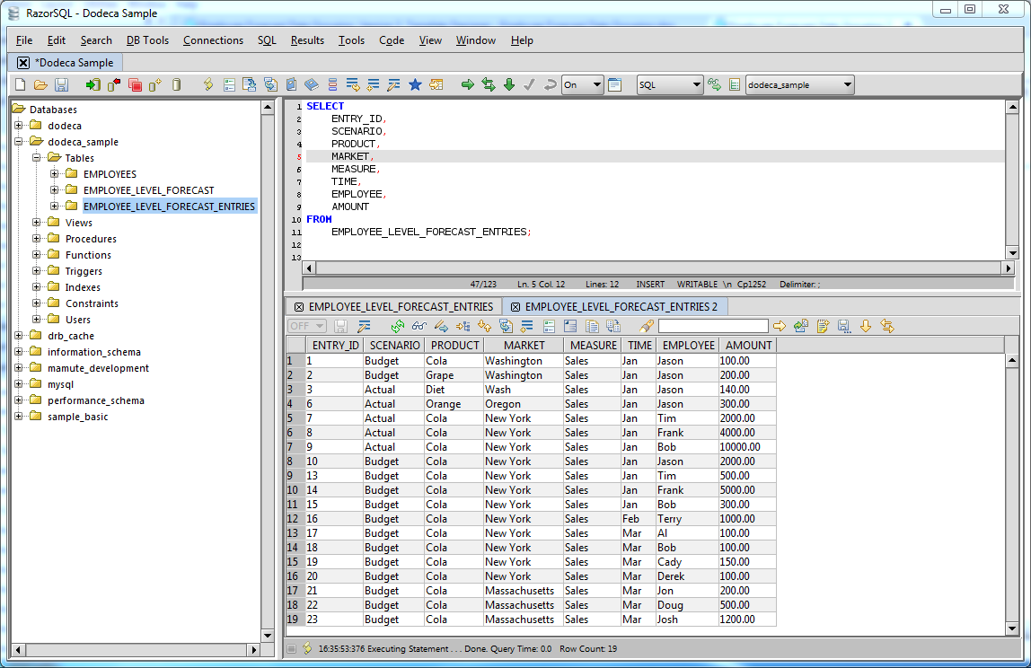
The SQL Server staging database is relatively simple.  There is now a table that will have the data loaded to it (this is the data that was loaded to the staging cube with a load rule).  The other tables include a list of financial pages (these are the departments on the sub-cubes, so to speak), a table for the list of databases (you’ll see why in a minute), a table for linking the departments/pages to a particular database, a table linking accounts to departments (pages), a page-roll table to manage the hierarchy of how pages aggregate to “bigger” pages, and a location/recap table that links the different small locations to their bigger parent locations (this is the equivalent of the location summing from the original staging database).

With all these tables in place, it’s time to add a few special views that will make life easier for us (and our load rules):

SELECT
     D.database_name
     , P.physical_page
     , A.account
     , K.div
     , K.yr
     , K.pd
     , K.amt
FROM
     account_dept AS A INNER JOIN
     jac_sum_vw AS K ON A.account = K.account INNER JOIN
     page P ON A.G_id = P.G_id INNER JOIN
     page_database AS G ON A.G_id = G.G_id INNER JOIN
     dbase AS D ON G.database_id = db.database_id

Obviously I didn’t provide the schema for the underlying tables, but this still should give you a decent idea of what’s going on.  There’s another view that sits on top of this one that takes care of the summing of locations for us, but it’s structurally similar to this one, so no surprises there.  What I end up with here is a view that has columns for the database name, the department, the account, location, year, period, and the amount.  So not only is this perfect for a fact table down the road when I convert this to EIS, I can also use the exact same view for all of my databases, and a very similar load rule in each database that simply references a different database.

This all took a day or two to setup, but after I started getting data how I wanted, I got pretty stoked that I was well on my way to boosting performance of this system.  One of the nice things about the way it’s setup in the relational database is also that it’s very flexible — extra databases, departments, locations, and anything else can be added to one central place without too much trouble.

Interestingly enough, this entire system is one that’s been in production for years but the “test” copy of things was sort of forgotten about and completely out of sync with production.  Since I was getting closer to the point where I was ready to load some cubes, I needed to sync test to prod (oddly enough) so I could do all testing without hosing things up.  Basically I just copied the apps from the production server to the test server with EAS, copied the existing automation folder, changed some server names and passwords (which were all hard-coded, brilliant…), and was pretty much good to go.   On a side note, I took the opportunity to rewrite the automation in modular, test-ready form (basically this involved cleaning up the old hard-coded paths and making it so I could sync test to prod much easier).

My next step was to design a load rule to load data up, to make sure that the structure of the tables and views was sufficient for loading data.  I did a normal SQL load rule that pulled data from the view I setup.  The load rule included some text replacements to adapt my version of departments to the actual alias name in the database, but otherwise didn’t need anything major to get working.  I loaded one period of data, calculated, saw that I was off a bit, researched some things, tweaked the load rule, recalculated, and so on, until finally the numbers were tying out with what I was seeing.  Not bad, not bad at all.

After this basic load rule was working correctly, I started gutting the automation system to clean things up a bit more and use the new load rule (with the old calcs).  After I felt good about the basic layout of things and got to the point where I was ready to copy this out to the other 18 or however many cubes.  Then I put some hooks in the automation to create a log file for me, so I can track performance.

For performance profiling, I used a technique that I’ve been using for awhile and have been quite happy with.  I have a small batch file in the automation folder called essprof.bat that has this in it:

@For /f "tokens=2-4 delims=/ " %%a in ('date /t') do @set FDATE=%%c-%%a-%%b
@echo %2,%FDATE% %TIME% >> %1

Basically when you call this file from another batch file, you tell it what file you want to append the data to, what the step should be named, and it takes care of the rest.  Here is how I might call it from the main automation script:

CALL essprof.bat %PROFFILE% START-PROCESS

The PROFFILE variable comes from a central configuration file and points to a location in the logging folder for this particular automation set.  For this particular line, I would get output like the following:

START-PROCESS,2009-07-31  8:57:09.18

The For loop in the batch file parses the DOS/shell date command a little bit, and together with the TIME variable, I get a nice timestamp — one that, incidentally, can be read by Excel very easily.

So what’s this all for?  As I did in the original performance chart, I want to profile every single step of the automation so I can see where I’m spending my time.  Once I filled out the rest of the load rules and ran the process a few times to work out the kinks, I now had a good tool for analyzing my performance.  Here is what one of the initial runs looked like:

start-db02-process 	10:54 AM
finish-db02-process 	10:54 AM
start-db03-process 	10:54 AM
finish-db03-process 	10:57 AM
start-db03GP-process 	10:57 AM
finish-db03GP-process 	10:58 AM
start-db04-process 	10:58 AM
finish-db04-process 	11:13 AM
start-db05-process 	11:13 AM
finish-db05-process 	11:13 AM
start-db06-process 	11:13 AM
finish-db06-process 	11:13 AM
start-db07A-process 	11:13 AM
finish-db07A-process 	11:13 AM
start-db07D-process 	11:13 AM
finish-db07D-process 	11:14 AM
start-db07L-process 	11:14 AM
finish-db07L-process 	11:14 AM
start-db07M-process 	11:14 AM
finish-db07M-process 	11:14 AM
start-db07T-process 	11:14 AM
finish-db07T-process 	11:14 AM
start-db08-process 	11:14 AM
finish-db08-process 	11:14 AM
start-db09-process 	11:14 AM
finish-db09-process 	11:14 AM
start-db10-process 	11:14 AM
finish-db10-process 	11:14 AM
start-db11-process 	11:14 AM
finish-db11-process 	11:14 AM
start-db12-process 	11:14 AM

And how do we look?  We’re chunking through most of the databases in about 20 minutes.  Not bad!  This is a HUGE improvement over the hour and a half processing time that we had earlier.  But, you know what, I want this to run just a little bit faster.  I told myself that if I was going to go to the trouble of redoing the entire, perfectly working automation system in a totally new format, then I wanted to get this thing down to FIVE minutes.

Where to start?

Well, first of all, I don’t really like these dense and sparse settings.  Scenario and time are dense and everything else is sparse.  For historical reasons, the Scenario dimension is kind of weird in that it contains the different years, plus a couple budget members (always for the current year), so it’s kind of like a hybrid time/scenario dimension.  But, since we’ll generally be loading in data all for the same year and period at once (keep in mind, this is a period-based process we’re improving), I see no need to have Scenario be dense. Having only one dense dimension (time) isn’t quite the direction I want to go in, so I actually decided to make location a dense dimension.  Making departments dense would significantly increase my inter-dimensional irrelevance so Location seems like a sensible choice — especially given the size of this dimension, which is some 20 members or so.  After testing out the new dense/sparse settings  on a couple of databases and re-running the automation, I was happy to see that not only did the DB stats look good, but the new setting was helping improve performance as well.  So I went ahead and made the same change to all of the other databases, then re-ran the automation to see what kind of performance I was getting.

End to end process time was now down to 12 minutes — looking better!  But I know there’s some more performance out there.  I went back to the load rule and reworked it so that it was “aligned” to the dense/sparse settings.  That is, I set it so the order of the columns is all the sparse dimensions first, then the dense dimensions.  The reason for this is that I want Essbase to load all the data to a single data block that it can, and try to minimize the number of times that the data block is loaded to memory.

Before going too much further I added some more logging to the automation so I could see exactly when the database process started, when it ran a clearing calc script, loaded data, and calculated again.

Now I was down to about 8 minutes… getting better.  As it turns out, I am using the default calculation for these databases, which is a CALC ALL, so that is a pretty ripe area for improvement.  Since I know I’m loading data all to one time period and year, and I don’t have any “fancy” calcs in the database, I can rewrite this to fix on the current year and period, aggregate the measures and departments dimensions, and calc on the location dimension.  By fancy, I’m referring to instances were a simple aggregation as per the outline isn’t sufficient — however, in this case, just aggregating works fine.  I rewrote the FIX, tested it, and rolled it out to all the cubes.  Total end to end load time was now at about four minutes.

But, this four minute figure was cheating a little since it didn’t include the load time to SQL, so I added in some of the pre-Essbase steps such as copying files, clearing out the SQL table, and loading in the data.  Fortunately, all of these steps only added about 15 seconds or so.

I decided to see if using a more aggressive threads setting to load data would yield a performance gain — and it did.  I tweaked essbase.cfg to explicitly use more threads for data loading (I started with four threads), and this got total process time down to just under three minutes (2:56).

As an aside, doing in three minutes what used to take 90 would be a perfectly reasonable place to stop, especially considering that my original goal was to get to five minutes.

But this is personal now.

Me versus the server.

I want to get this thing down to a minute, and I know I still have some optimizations left on the table that I’m not using.  I’ve got pride on the line and it’s time to shave every last second I can out of this thing.

Let’s shave a few more seconds off…

Some of the databases don’t actually have a departments dimension but I’m bringing a “dummy” department just so my load rules are all the same — but why bring in a column of data I don’t need?   Let’s tweak that load rule to skip that column (as in, don’t even bother to bring it in from SQL) on databases that don’t have the departments dimension.  So I tweaked the load rule got the whole process down to 1:51.

Many of these load rules are using text replacements to conform the incoming department to something that is in the outline… well, what if I just setup an alternate alias table so I don’t even have to worry about the text replacements?  It stands to reason, from an Essbase data load perspective, that it’s got to cycle through the list of rows on the text replace list and check it against the incoming data, so if I can save it the trouble of doing that, it just might go faster.  And indeed it does: 1:39 (one minute, thirty nine seconds).  I don’t normally advocate just junking up the outline with extra alias tables, but it turns out that I already had an extra one in there that was only being used for a different dimension, so I added my “convenience” aliases to that.  I’m getting close to that minute mark, but of course now I’m just shaving tiny bits off the overall time.

At this point, many of the steps in the 90-step profiling process are taking between 0 and 1 seconds (which is kind of funny, that a single step starts, processes, and finishes in .3 seconds or something), but several of them stand out and take a bit longer.  What else?

I tried playing with Zlib compression, thinking that maybe if I could shrink the amount of data on disk, I could read it faster into memory.  In all cases this seemed to hurt performance a bit so I went back to bitmap.  I have used Zlib compression quite successfully before, but there’s probably an overhead hit I’m taking for using it on relatively “small” database — in this case I need to get in and get out as fast as I can and bitmap seems to allow me to do that just a little faster, so no Zlib this time around (but I still love you Zlib, no hard feelings okay?).

Okay, what ELSE?  I decided to bump the threads on load to 8 to see if I got more of a boost — I did.  Total load time is now at 1:25.

The SQL data load using bcp (the bulk load command line program) takes up a good 10 seconds or so, and I was wondering if I could boost this a bit.  bcp lets you tweak the size of the packets, number of rows per batch, and lock the table you’re loading to.  So I tweaked the command line to use these options, and killed another few seconds off the process — down to 1:21.

Now what?  It turns out that my Location dimension is relatively flat, with just two aggregated members in it.  I decided that I don’t really need to calculate these and setting them as dynamic would be feasible.  Since location is dense this has the added benefit of removing two members from my stored data block, or about 10 percent in this case.  I am definitely approaching that area where I am possibly trading query performance just for a little bit faster load, but right now I don’t think I’m trading away any noticeable performance on the user side (these databases are relatively small).

Just reducing the data blocks got me down to 1:13 or so (closer!), but since there are now no aggregating members that are stored in the Location dimension, I don’t even need to calculate this dimension at all — so I took the CALC DIMs out of all the calc scripts and got my calc time down further to about 1:07.

Where oh where can I find just 7 more seconds to shave off?  Well, some of these databases also have a flat department structure, so I can definitely shave a few seconds and save myself the trouble of having to aggregate the departments dimension by also going to a dynamic calc on the top level member.  So I did this where I could, and tweaked the calcs accordingly and now the automation is down to about 1:02.

And I am seriously running out of ideas as to where I can shave just a COUPLE of more seconds off.  Come on Scotty, I need more power!

Well, keeping in mind that this is a period process that runs numerous times during closing week, part of this process is to clear out the data for the current period and load in the newer data.  Which means that every database has a “clear” calc script somewhere.  I decided to take a look at these and see if I could squeeze a tiny bit of performance out.

I wanted to use CLEARBLOCK because I’ve used that for good speedups before, but it’s not really effective as a speedup here because I have a dense time dimension and don’t want to get rid of everything in it (and I think CLEARBLOCK just reverts to a normal CLEARDATA if it can’t burn the whole block).  However, there were still some opportunities to tweak the clearing calc script a little so that it was more conducive to the new dense and sparse settings.   And sure enough, I was able to shave .1 or .2 seconds off of the clear calc on several databases, giving me a total process time of……. 59.7 seconds.   Made it, woot!

Along the way I tried several other tweaks here and there but none of them gave me a noticeable performance gain.  One change I also made but seems to be delivering sporadic speed improvements is to resize the index caches to accommodate the entire index file.  Many of the indexes are less than 8 megabytes already so they’re fine in that regard, some of them aren’t so I sized them accordingly.  I’d like to believe that keeping the index in memory is contributing to better performance overall but I just haven’t really been able to profile very well.

After all that, in ideal circumstances, I got this whole, previously hour-and-a-half job down to a minute.  That’s not bad.  That’s not bad at all.  Sadly, my typical process time is probably going to be a minute or two or longer as I adjust the automation to include more safety checks and improve robustness as necessary.  But this is still a vast improvement.  The faster turnaround time will allow my users to have more accurate data, and will allow me to turn around the databases faster if something goes wrong or I need to change something and update everything.  In fact, this came in extremely useful today while I was researching some weird variances against the financial statements.  I was able to make a change, reprocess the databases in a minute or so, and see if my change fixed things.  Normally I’d have to wait an hour or more to do that. I may have optimized more than I needed to (because I have an almost unhealthy obsession with performance profiling and optimization), but I think it was worth it.  The automation runs fast.

So, my advice to you: always look at the big picture, don’t be afraid to use a different technology, get metrics and refer to them religiously (instead of “hmm, I think it’s faster this way), try to think like Essbase — and help it do its job faster, and experiment, experiment, experiment. Continue Reading…

Essbase and SQL Server Express: just don’t

I’m working on a writeup on how to get a fully functional Essbase server up and running in a virtual machine (using Sun VirtualBox).  I’m currently working on the steps — setting up the Essbase funtionality is relatively straightforward, although you need a relational database to store various information.

“No problem,” I thought to myself, “I’ll just pop on a copy of SQL Server Express.” Oh how naive I was.  In theory, I’m sure it’s possible to use SQL Server Express as the backend for a Hyperion installation, but after fiddling around with various options, enabling TCP/IP, and doing everything else I could think of, I just couldn’t get things to work.  So I yanked it off the virtual machine and put the real deal on — a full copy of SQL Server 2005 — and presto!  I was up and running in no time.  So if you happen to reach this blog article because you googled “SQL Server Express Essbase oh for the love of god why do you mock me” or something similar, I hope this popped first to let you know you may be in for a bumpy ride.

Update: Several of my readers have commented on how they’ve been successfully using SQL Server Express for their purposes.  I didn’t spend an incredible amount of time trying to configure Express to work, and given that the full version of SQL Server is available to me, I went ahead and installed that without looking back.  As I suspected, you need to play with the connection settings a bit in order to get things to work, and if someone cares to do a writeup of what that procedure looks like, I’d be more than happy to post it here.  Thanks for the suggestions, all.

Essbase Performance Optimization: it’s not just the calc script

Here’s a quick post that is a bit of a precursor to some of my more in-depth performance analysis articles that will be coming out in the future.  One of my automation systems takes a bit over an hour to run.  There are a lot of people I know that need to squeeze performance out of their systems and immediately look to their calc scripts.  Yes, calc time can be a large part of your downtime, as can data loads, reports, and other activities.  But I always stress that it is useful and important to understand your systems in their entirety.

As part of looking at the bigger picture, I put together the following graph showing each step and how long it takes in this system that takes around an hour.  It’s not hard to tell that the majority of the time that it takes to run this job (the brownish bar that takes about an hour) is in one task!  And what is that task?  It’s a bunch of report scripts running on a staging database.  This is clearly an obvious place for me to look at ways of saving time.

Duration of Steps for an Essbase Automation Process

Duration of Steps for an Essbase Automation Process

The staging database is is a rather clever cube that is essentially used to scrub, aggregate, and associate raw account level data to some more meaningful dimensional combinations for all of the other databases.  Data comes in, it’s calculated, and it outputs a bunch of report scripts.  Fundamentally, the reason that this approach takes so much time is that there are two highly sparse dimension combinations with tens of thousands of members each, and the report script writer has to go through a ton of on-disk data in order to figure out what to write.  I could spend some time trying to optimize this process, in fact, I could probably play with some settings and get at least 20% improvement right now.

But, this is one of those times where it pays to stand back and look at what we’re trying to accomplish.  As it turns out, I actually have all of the infrastructure I need to accomplish this task, but it’s in a SQL database.  And, the task that is being performed is actually much more conducive to the way that a relational database works.  I’m still putting the finishing touches on this process, but it’s mostly complete as of right now, and the performance is amazing.  I can pump through the same amount of data in mere minutes now, with no loss of functionality.

My specific goal is to get this process that takes an hour or longer, to run in less than five minutes.  I chose this instead of “as fast as possible” because I wanted something concrete and attainable.  (My secret goal, just for kicks, is to get this all to run in under a minute).  Once the automation for the SQL staging is all in place, I will be going through all of the individual databases and tweaking any and all settings in order to shave their downtime as well.

Historically, not a lot of effort has gone into extensive profiling on these cubes, so as nerdy as it sounds, I’m actually very interested to see where else I can shave a few seconds off.  At first this will undoubtedly involve using more write threads in the dataload, rewriting the calc scripts to tighten them up from just their current CALC ALL, aligning the order of the data fields and rows with the dense/sparse-ness of the outlines and the outline order, choosing better cache settings that are customized for the size of the index and page files, and perhaps looking at benefits of zlib compression (theoretically more CPU time to compress/decompress, however, generally the CPUs on these servers are not slammed very hard, so if I can get the size of the physical page files down, I may be able to read it into memory faster).

So remember — you spend a lot of time doing calculations, but that might not alway be where the low hanging fruit is.  I cannot stress enough the importance of understanding where you spend your time, and using that as a basis for helping Essbase do its job faster.

An Introduction Essbase Integration Services (EIS)

So, just what is this EIS thing?  You’ve heard about it, you know it has something to do with outlines, but you haven’t used it and you just don’t know where to start.  I understand.  I’ve been there.  I couldn’t really see an immediate payoff to using it, which kind of made getting all setup a little more daunting.  Please note that this article is written referring mostly to version 7 of EIS — I’m not sure what changes may have occurred since then.

Interestingly, my motivation for using EIS was a bit odd.  I was building some new cubes for the enterprise and they were in ASO for the first time.  The cubes were the evolution of a set of cubes that had been around in the company for a number of years, and the goal was to take what worked (and avoid what didn’t), and apply it for the entire organization.  Which is huge.  Hence the reason for ASO.  Along with learning all of the quirks that ASO brings to the table versus BSO, I also ran into another issue.  The original cubes, as part of their calculation method, would FIX on all of the accounts related to Gross Profit, flip the sign, and then roll up the whole cube.  The reason for this is that the GP accounts come in their “natural” accounting sign, so something like a sales account would be negative in the source database.  But since there are no calc scripts in ASO, I had to come up with another solution.  Well, it turns out that there’s this neat little feature on load rules that lets you flip the sign on a particular UDA.

Given that the Accounts dimension changes from period to period (and has  a bajillion members in it), it was necessary to come up with a mechanism to tag all of the appropriate accounts with the UDA I needed.  I got this working just fine with a load rule, ran it, and voila, I had a nice shiny UDA called “GP” on the members I needed.  I was feeling pretty pleased with myself… until the next time I ran the automation.  I ran it again and again for testing purposes.  And when I cracked open the outline again in EAS, I noticed that my members had about 20 copies of the “GP” UDA on them.

As it turns out, I believe this was a bonafide bug in Essbase 7.x that was fixed at some point — at the time I was writing the automation I believe my servers were 7.1.2.  But at the time we had no plans to put in the point upgrade, and not being the kind of guy that likes to wait around anyway, I decided to take the somewhat unconventional approach and just implement the entire thing in EIS.  So, you can honestly say that my entire reason for picking up EIS is because my UDAs were multiplying like tribbles on me, but that’s life, funny things like that happen.

So, getting back to the main idea here, what exactly is EIS?  In short, it’s a tool for creating outlines based on relational data.  It essentially takes the place of editing your outlines in EAS, using dimension build Load rules.  You can also load data through EIS (although I typically decline to do so and instead automate it with MaxL elsewhere).  And, unlike EAS with it’s oh-why-don’t-you-just-stab-me-in-the-eyes-already interface, EIS has a pretty slick interface.  In fact, the interface is so nice, it makes me just a little bit tingly on the inside… but then again that could just be related to my unnatural obsession with all things multi-dimensional.

Why use EIS?  Once you get good at it, and have some good upstream data to work with, you can crank out some outlines pretty fast.  You can also keep them updated very easily, by virtue of updating the source relational data that EIS reads.  I’m also completely and utterly sick of whipping up new load rules to update dimensions.  In the case of some of my attribute dimensions, I can’t even imagine the pain I would have to go through to implement the same functionality with a load rule.  EIS is also the tool you’ll need to use to link up to some drill-through data.

To get started with EIS, you need to make sure that EIS is installed on a server somewhere.  I just have mine running on the Essbase server itself and I find I am happy with this approach.  EIS will store all of it’s data in something referred to as the “metadata catalog,” which is just a SQL database that you’ll need to setup.  Oddly enough, when I started using EIS, I didn’t actually know I had a SQL server, but I figured there was one somewhere, so I started pinging things, and behold, I found a SQL box laying around (I guess the proper way of doing this would be to fill out a capital appropriations request for a server or something, but this makes a way better story).  It’s a SQL Server box with modest specs, but it gets the job done just fine.  It’s also the same server that I use to hold all of the relational data that I use for building outlines.

In a nutshell, you need to create a new database, then use one of the scripts that comes with EIS in order to populate the new database with some initial data.  This data is simply something that EIS will use under the hood and you won’t have to (and shouldn’t) edit the data by hand once you get it all loaded up.  After you have the shell of the metadata catalog setup, you will need to define some data sources from the EIS server to your relational data.  In my case, with Windows servers, this meant just setting up an ODBC connection on the Essbase server and pointing it to another new SQL database on the SQL server.

At this point, I would highly recommend following the EIS instructions and setting up the data they include for TBC (The Beverage Company).  Setting up this example means that you will be setup with the EIS Model for TBC, as well as a metaoutline for TBC.

In EIS terminology, you create a model first, then a metaoutline.  A model is something you create in order to link together your SQL tables and tell EIS how they relate to each other.  At the center of this model you will have a Fact Table.  You can sort of think of the Fact Table as being similar in nature to the type of data that you would load to your Essbase cube with a normal load rule.  For example, if the rows in your data file had fields for the scenario, year, time period, location, department, measure, then a dollar amount or other figure, you can think of this as your fact table.  In this case, think of the different time periods for a moment.  In a typical periods/quarters/year setup, your text file would just have an 01 for period 01, an 02 for period 02, and so on.  Generally the source data wouldn’t make any sort of mention of the quarters, for example,  but EIS needs to know about this.  On the model, you would link the Period on the fact table to another table in your relational database that shows how to build the Time dimension based on that data.

The metaoutline has to be created after the model, because it is highly dependant on the way the model is setup.  In fact, when you create the metaoutline, you tell EIS which model to base it off of.  As the seasoned EIS veterans know about models and metaoutlines, once you commit to something in the model, you are basically married to it.  You can’t go around gutting the model too much unless you first make changes to your metaoutline(s).

If you’ve setup the model in a sane manner, you can then use the dimensions/tables you defined sort of as Lego blocks in your metaoutline, you can mix and match different dimensions and come up with a working outline.  You can even create arbitrary members in dimensions or completely new dimensions, if that’s what you need for that particular outline.  Try your best to keep it in the model though — it’ll usually pay off in the long run.

With the metaoutline properly defined, you can then load the members to a cube.  This is a straightforward process (assuming everything is setup correctly) where EIS will take your metaoutline, which is in turn based off your model, which is in turn based off your relational (SQL) data, and build a completely fresh outline for you.  Of course, this process can be automated (as with just about everything else).  If you’ve built everything correctly you can also load data through EIS too, although in practice I tend to find myself leaving that to an automation system, but it’s always good to know that your models are built properly.

The barriers to entry for setting up EIS can be daunting if you aren’t already using it.  You have to install it on a server, setup a SQL database for the metadata catalog, have some source data in SQL that you want to use to build/load outlines (which may require you to brush up on your SQL skills if you’re a bit rusty), and figure out how the tool works.  As always, learning from examples and experimenting on your own are very good ways to go — so if you can get the EIS demo app installed you should be able to see how things are put together.  The payoff though, for using EIS, can be immense.  You don’t have to mess around with all those dimension build load rules, you can spin up new outlines in a jiffy (without necessarily reinventing the wheel everytime), and girls think it’s pretty cool (and for all you female cube geeks out there, I’m sure the guys will be impressed too).

If you’re still curious about EIS (and who wouldn’t be?), feel free to drop me a line.  Also, if you’d like to see more articles about EIS, let me know and I get dig into some of the more complex stuff.  The screenshots below show some EIS screens — a model, a metaoutline, and building an outline from a metaoutline.   See in the model how the fact table is in the middle, with some other dimensions attached to it.  I blurred out some server information, but it doesn’t affect the purpose of the screenshot.