The Old
In many companies, there is a lot of code laying around that is, for lack of better word, “old.” In the case of Essbase-related functionality, this may mean that there are some automation systems with several ESSCMD scripts laying around. You could rewrite them in MaxL, but where’s the payoff? There is nothing inherently bad with old code, in fact, you can often argue a strong case to keep it: it tends to reflect many years of tweaks and refinements, is well understood, and generally “just works” — and even when it doesn’t you have a pretty good idea where it tends to break.
Rewrite it?
That being said, there are some compelling reasons to do an upgrade. The MaxL interpreter brings a lot to the table that I find incredibly useful. The existing ESSCMD automation system in question (essentially a collection of batch files, all the ESSCMD scripts with the .aut extension, and some text files) is all hard-coded to particular paths. Due to using absolute paths with UNC names, and for some other historical reasons, there only exists a production copy of the code (there was perhaps a test version at some point, but due to all of the hard-coded things, the deployment method consisted of doing a massive search and replace operation in a text editor). Because the system is very mature, stable, and well-understood, it has essentially been “grandfathered” in as a production system (it’s kind of like a “black box” that just works).
The Existing System
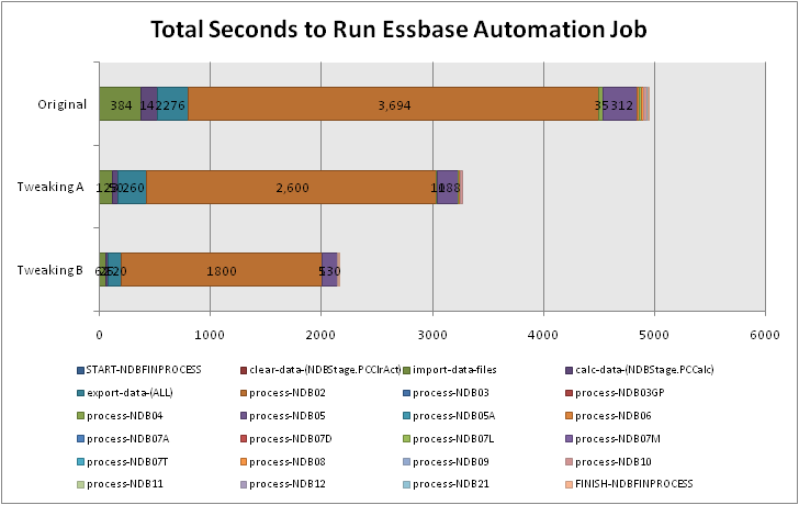
The current system performs several different functions across its discreet job files. There are jobs to update outlines, process new period data, perform a historical rebuild of all cubes (this is currently a six hour job and in the future I will show you how to get it down to a small fraction of its original time), and some glue jobs that scurry data between some different cubes and systems. The databases in this system are setup such that there are about a dozen very similar cubes. They are modeled on a series of financial pages, but due to differences in the way some of the pages work, it was decided years ago that the best way to model cubes on the pages was to split them up in to different sets of cubes, rather than one giant cube. This design decision had paid off in many ways. One, it keeps the cubes cleaner and more intuitive; interdimensional irrelevance is also kept to a minimum. Strategic dense/sparse settings and other outline tricks like dynamic calcs in the Time dimension rollups also keep things pretty tight.
Additionally, since the databases are used during the closing period, not just after (for reporting purposes), new processes can go through pretty quickly and update the cubes to essentially keep them real-time with how the accounting allocations are being worked out. Keeping the cubes small allows for a lot less down-time (although realistically speaking, even in the middle of a calc, read-access is still pretty reliable).
So, first things first. Since there currently are no test copies of these “legacy” cubes, we need to get these setup on the test server. This presents a somewhat ironic development step: using EAS to copy the apps from the production server, to the development server. These cubes are not spun up from EIS metaoutlines, and there is very little compelling business reason to convert them to EIS just for the sake of converting them, so this seems to be the most sensible approach.
Although the outlines are in sync right now between production and development because I just copied them, the purpose of one of the main ESSCMD jobs is to update the outlines on a period basis, so this seems like a good place to start. The purpose of the outline update process is basically to sync the Measures dimension to the latest version of the company’s internal cross-reference. The other dimensions are essentially static, and only need to be updated rarely (e.g., to add a new year member). The cross-reference is like a master list of which accounts are on which pages and how they aggregate.
On a side note, the cross-reference is part of a larger internal accounting system. What it lacks in flexibility, it probably more than makes up for with reliability and a solid ROI. One of the most recognized benefits that Essbase brings to the table in this context is a completely new and useful way of analyzing existing data (not to mention write-back functionality for budgeting and forecasting) that didn’t exist. Although Business Objects exists within the company too, it is not recognized as being nearly as useful to the internal financial customers as Essbase is. I think part of this stems from the fact that BO seems to be pitched more to the IT crowd within the organization, and as such, serves mostly as a tool to let them distribute data in some fashion, and call it a day. Essbase really shines, particularly because it is aligned with the Finance team, and it is customized (by finance team members) to function as a finance tool, versus just shuttling gobs of data from the mainframe to the user.
The cross-reference is parsed out in an Access database in order to massage the data into various text files that will serve as the basis of dimension build load rules for all the cubes. I know, I know, I’m not a huge Access fan either, but again, the system has been around forever, It Just Works, and I see no compelling reason to upgrade this process, to say, SQL Server. Because of how many cubes there are, different aliases, different rollups, and all sorts of fun stuff, there are dozens of text files that are used to sync up the outlines. This has resulted in some pretty gnarly looking ESSCMD scripts. They also use the BEGININCBUILD and ENDINCBUILD ESSCMD statements, which basically means that the cmd2mxl.exe converter is useless to us. But no worries — we want to make some more improvements besides just doing a straight code conversion.
In a nutshell, the current automation script logs in (with nice hard-coded server path, user name, and password, outputs to a fixed location, logs in to each database in sequence, and has a bunch of INCBUILDDIM statements. ESSCMD, she’s an old girl, faithful, useful, but just not elegant. You need a cheatsheet to figure out what the invocation parameters all mean. I’ll spare you the agony of seeing what the old code looks like.
Goals
Here are my goals for the conversion:
- Convert to MaxL. As I mentioned, MaxL brings a lot of nice things to the table that ESSCMD doesn’t provide, which will enable some of the other goals here.
- Get databases up and running completely in test — remember: the code isn’t bad because it’s old or “legacy code,” it’s just “bad” because we can’t test it.
- Be able to use same scripts in test as in production. The ability to update the code in one place, test it, then reliably deploy it via a file-copy operation (as opposed to hand-editing the “production” version) is very useful (also made easier because of MaxL).
- Strategically use variables to simplify the code and make it directory-agnostic. This will allow us to easily adapt the code to new systems in the future, for example, if we want to consolidate to a different server in the future, even one on a different operating system).
- And as a tertiary goal: Start using a version control system to manage the automation system. This topic warrants an article all on itself, which I fully intend to write in the future. In the meantime, if you don’t currently use some type of VCS, all you need to know about the implications of this are that we will have a central repository of the automation code, which can be checked-in and checked-out. In the future we’ll be able to look at the revision history of the code. We can also use the repository to deploy code to the production server. This means that I will be “checking-out” the code to my workstation to do development, and I’m also going to be running the code from my workstation with a local copy of the MaxL interpreter. This development methodology is made possible in part because in this case, my workstation is Windows, and so are the Essbase servers.
For mostly historical reasons the old code has been operated and developed on the analytic server itself, and there are various aspects about the way the code has been developed that mean you can’t run it from a remote server. As such, there are various semantic client/server inconsistencies in the current code (e.g. in some cases we are referring to a load rule by it’s App/DB context, and in some cases we are using an absolute file path). Ensuring that the automation works from a remote workstation will mean that these inconsistencies are cleaned up, and if we choose to move the automation to a separate server in the future, it will be much easier.
First Steps
So, with all that out of the way, let’s dig in to this conversion! For the time being we’ll just assume that the versioning system back-end is taken care of, and we’ll be putting all of our automation files in one folder. The top of our new MaxL file (RefreshOutlines.msh) looks like this:
msh "conf.msh";
msh "$SERVERSETTINGS";
What is going on here? We’re using some of MaxL features right away. Since there will be overlap in many of these automation jobs, we’re going to put a bunch of common variables in one file. These can be things like folder paths, app/database names, and other things. One of those variables is the $SERVERSETTINGS variable. This will allow us to configure a variable within conf.msh that points to where the server-specific MaxL configuration file. This is one method that allows us to centralize certain passwords and folder paths (like where to put error files, where to put spool files, where to put dataload error files, and so on). Configuring things this way gives us a lot of flexibility, and further, we only really need to change conf.msh in order to move things around — everything else builds on top of the core settings.
Next we’ll set a process-specific configuration variable which is a folder path. This allows us to define the source folder for all of the input files for the dimension build datafiles.
SET SRCPATH = "../../Transfer/Data";
Next, we’ll log in:
login $ESSUSER identified by $ESSPW on $ESSSERVER;
These variables are found in the $SERVERSETTINGS file. Again, this file has the admin user and password in it. If we needed more granularity (i.e., instead of running all automation as the god-user and instead having just a special ID for the databases in question), we could put that in our conf.msh file. As it is, there aren’t any issues on this server with using a master ID for the automation.
spool stdout on to "$LOGPATH/spool.stdout.RefreshOutlines.txt";
spool stderr on to "$LOGPATH/spool.stderr.RefreshOutlines.txt";
Now we use the spooling feature of MaxL to divert standard output and error output to two different places. This is useful to split out because if the error output file has a size greater than zero, it’s a good indicator that we should take a look and see if something isn’t going as we intended. Notice how we are using a configurable LOGPATH directory. This is the “global” logpath, but if we wanted it somewhere else we could have just configured it that way in the “local” configuration file.
Now we are ready for the actual “work” in this file. With dimension builds, this is one of the areas where ESSCMD and MaxL do things a bit differently. Rather than block everything out with begin/end build sections, we can jam all the dimension builds into one statement. This particular example has been modified from the original in order to hide the real names and to simplify it a little, but the concept is the same. The nice thing about just converting the automation system (and not trying to fix other things that aren’t broken — like moving to an RDBMS and EIS) is that we get to keep all the same source files and the same build rules.
import database Foo.Bar dimensions

    from server text data_file "$SRCPATH/tblAcctDeptsNon00.txt"
    using server rules_file 'DeptBld' suppress verification,

    from server text data_file "$SRCPATH/tblDept00Accts.txt"
    using server rules_file 'DeptBld'

    preserve all data
    on error write to "$ERRORPATH/JWJ.dim.Foo.Bar.txt";
In the actual implementation, the import database blocks go on for about another dozen databases. Finally, we finish up the MaxL file with some pretty boilerplate stuff:
spool off;
logout;
exit;
Note that we are referring to the source text data file in the server context. Although you are supposed to be able to use App/database naming for this, it seems that on 7.1.x, even if you start the filename with a file separator, it still just looks in the folder of the current database. I have all of the data files in one place, so I was able to work around this by just changing the SRCPATH variable to go up two folders from the current database, then back down into the Transfer\Data folder. The Transfer\Data folder is under the Essbase app\ folder. It’s sort of a nexus folder where external processes can dump files because they have read/write access to the folder, but it’s also the name of a dummy Essbase application (Transfer) and database (Data) so we can refer to it and load data from it, from an Essbase-naming perspective. It’s a pretty common Essbase trick. We are also referring to the rules files from a server context. The output files are to a local location. This all means that we can run the automation from some remote computer (for testing/development purposes), and we can run it on the server itself. It’s nice to sort of “program ahead” for options we may want to explore in the future.
For the sake of completeness, when we go to turn this into a job on the server, we’ll just use a simple batch file that will look like this:
cd /d %~dp0
essmsh RefreshOutlines.msh
The particular job scheduling software on this server does not run the job in the current folder of the job, therefore we use cd /d %~dp0 as a Windows batch trick to change folders (and drives if necessary) to the folder of the current file (that’s what %~dp0 expands out to). Then we run the job (the folder containing essmsh is in our PATH so we can run this like any other command).
All Done
This was one of the trickier files to convert (although I have just shown a small section of the overall script). Converting the other jobs is a little more straightforward (since this is the only one with dimension build stuff in it), but we’ll employ many of the same concepts with regard to the batch file and the general setup of the MaxL file.
How did we do with our goals? Well, we converted the file to MaxL, so that was a good start. We copied the databases over to the test server, which was pretty simple in this case. Can we use the same scripts in test/dev and production? Yes. Since the server specific configuration files will allow us to handle any folder/username/password issues that are different between the servers, but the automation doesn’t care (it just loads the settings from whatever file we tell it), I’d say we addressed this just fine. We used MaxL variables to clean things up and simplify — this was a pretty nice cleanup over the original ESSCMD scripts. And lastly, although I didn’t really delve into it here, this was all developed on a workstation (my laptop) and checked in to a Subversion repository, further, the automation all runs just fine from a remote client. If we ever need to move some folders around, change servers, or make some other sort of change, we can probably adapt and test pretty quickly.
All in all, I’d say it was a pretty good effort today. Happy holidays ya’ll.